

前言:
什么是迁移学习(Transfer Learning)?简单的理解就是使用一些已经训练好的模型迁移到类似的新的问题进行使用,而不必对新问题重新建模,从头训练和优化参数。这些训练好的模型同时包含了优化好的参数,在使用的时候只需要做一些简单的调整就可以应用到新问题中了。
本文需要解决的问题使用了迁移过来的VGG16模型,本文最终会得到一个能对猫狗图片进行辨识的CNN(卷积神经网络),测试集用来验证我的模型是否能够很好的工作。
使用PyTorch搭建迁移学习模型:
VGG是由K. Simonyan和A. Zisserman 在论文 《Very Deep Convolutional Networks for Large-Scale Image Recognition》中创建的一种CNN(卷积神经网络)模型。该模型在 ImageNet:ImageNet(对百万级图片进行分类的比赛)挑战中取得过辉煌战绩。
VGG16模型的结构,如下图:
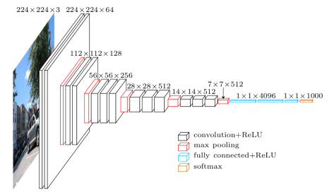
从图中可以看出,模型包括了多个卷积层、池化层、全连接层,作为输入的是一个224*224*3的图片(224*224位分辨率,3为RGB3个通道),输出是包含1000个分类的结果(本文只是做两个分类的应用,所以需要对最后一层进行改写)。使用PyTorch下载模型和参数很方便,使用方法如下:
from torchvision import models
model = models.vgg16(pretrained=True)
pretrained设置为True,程序会自动下载已经训练好的参数。
本为使用迁移学习实现猫狗图片的分类,数据集自来自Kaggle的一个比赛:Dogs vs. Cats Redux: Kernels Edition。
首先做图片的导入和预览,代码如下:
path = "dog_vs_cat"
transform = transforms.Compose([transforms.CenterCrop(224),
                                transforms.ToTensor(),
                                transforms.Normalize([0.5,0.5,0.5], [0.5,0.5,0.5])])

data_image = {x:datasets.ImageFolder(root = os.path.join(path,x),
                                     transform = transform)
              for x in ["train", "val"]}

data_loader_image = {x:torch.utils.data.DataLoader(dataset=data_image[x],
                                                batch_size = 4,
                                                shuffle = True)
                     for x in ["train", "val"]}
因为输入的图片需要分辨率为224*224,所以使用transforms.CenterCrop(224)对原始图片进行裁剪。载入的图片训练集合为20000和验证集合为5000(原始图片全部为训练集合,需要自己拆分出一部分验证集合),输出的Label,1代表是狗,0代表的猫。
X_train, y_train = next(iter(data_loader_image["train"]))
mean = [0.5,0.5,0.5]
std  = [0.5,0.5,0.5]
img = torchvision.utils.make_grid(X_train)
img = img.numpy().transpose((1,2,0))
img = img*std+mean

print([classes[i] for i in y_train])
plt.imshow(img)
['cat', 'dog', 'cat', 'dog']
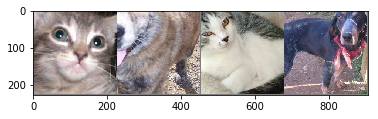
上图可以看出来,将要训练图片都是224*224*3。
迁移模型然后打印出模型的结构:
model = models.vgg16(pretrained=True)
print(model)
VGG (
  (features): Sequential (
    (0): Conv2d(3, 64, kernel_size=(3, 3), stride=(1, 1), padding=(1, 1))
    (1): ReLU (inplace)
    (2): Conv2d(64, 64, kernel_size=(3, 3), stride=(1, 1), padding=(1, 1))
    (3): ReLU (inplace)
    (4): MaxPool2d (size=(2, 2), stride=(2, 2), dilation=(1, 1))
    (5): Conv2d(64, 128, kernel_size=(3, 3), stride=(1, 1), padding=(1, 1))
    (6): ReLU (inplace)
    (7): Conv2d(128, 128, kernel_size=(3, 3), stride=(1, 1), padding=(1, 1))
    (8): ReLU (inplace)
    (9): MaxPool2d (size=(2, 2), stride=(2, 2), dilation=(1, 1))
    (10): Conv2d(128, 256, kernel_size=(3, 3), stride=(1, 1), padding=(1, 1))
    (11): ReLU (inplace)
    (12): Conv2d(256, 256, kernel_size=(3, 3), stride=(1, 1), padding=(1, 1))
    (13): ReLU (inplace)
    (14): Conv2d(256, 256, kernel_size=(3, 3), stride=(1, 1), padding=(1, 1))
    (15): ReLU (inplace)
    (16): MaxPool2d (size=(2, 2), stride=(2, 2), dilation=(1, 1))
    (17): Conv2d(256, 512, kernel_size=(3, 3), stride=(1, 1), padding=(1, 1))
    (18): ReLU (inplace)
    (19): Conv2d(512, 512, kernel_size=(3, 3), stride=(1, 1), padding=(1, 1))
    (20): ReLU (inplace)
    (21): Conv2d(512, 512, kernel_size=(3, 3), stride=(1, 1), padding=(1, 1))
    (22): ReLU (inplace)
    (23): MaxPool2d (size=(2, 2), stride=(2, 2), dilation=(1, 1))
    (24): Conv2d(512, 512, kernel_size=(3, 3), stride=(1, 1), padding=(1, 1))
    (25): ReLU (inplace)
    (26): Conv2d(512, 512, kernel_size=(3, 3), stride=(1, 1), padding=(1, 1))
    (27): ReLU (inplace)
    (28): Conv2d(512, 512, kernel_size=(3, 3), stride=(1, 1), padding=(1, 1))
    (29): ReLU (inplace)
    (30): MaxPool2d (size=(2, 2), stride=(2, 2), dilation=(1, 1))
  )
  (classifier): Sequential (
    (0): Linear (25088 -> 4096)
    (1): ReLU (inplace)
    (2): Dropout (p = 0.5)
    (3): Linear (4096 -> 4096)
    (4): ReLU (inplace)
    (5): Dropout (p = 0.5)
    (6): Linear (4096 -> 1000)
  )
)
可以看出模型的结构和最开始展示的VGG16图片结构是一样的,只是这里还包含了模型每层中实际需要传递的参数,想要迁移过来的VGG16模型适应新的需求,达到对猫狗图片很好的识别,需要改写VGG16的全连接层的最后一部分并且重新训练参数(即使只是训练整个全连接层的全部参数,普通的电脑也会花费大量的时间,所以这里只训练全连接层的最后一层),就能达到很好的效果了:
for parma in model.parameters():
    parma.requires_grad = False

model.classifier = torch.nn.Sequential(torch.nn.Linear(25088, 4096),
                                       torch.nn.ReLU(),
                                       torch.nn.Dropout(p=0.5),
                                       torch.nn.Linear(4096, 4096),
                                       torch.nn.ReLU(),
                                       torch.nn.Dropout(p=0.5),
                                       torch.nn.Linear(4096, 2))

for index, parma in enumerate(model.classifier.parameters()):
    if index == 6:
        parma.requires_grad = True

if use_gpu:
    model = model.cuda()


cost = torch.nn.CrossEntropyLoss()
optimizer = torch.optim.Adam(model.classifier.parameters())
parma.requires_grid = False目的是冻结参数,即使发生新的训练也不会进行参数的更新。
这里还对全连接层的最后一层进行了改写,torch.nn.Linear(4096, 2)使得最后输出的结果只有两个(只需要对猫狗进行分辨就可以了)。
optimizer = torch.optim.Adam(model.classifier.parameters())只对全连接层参数进行更新优化,loss计算依然使用交叉熵。
对改写后的模型进行查看:
VGG (
  (features): Sequential (
    (0): Conv2d(3, 64, kernel_size=(3, 3), stride=(1, 1), padding=(1, 1))
    (1): ReLU (inplace)
    (2): Conv2d(64, 64, kernel_size=(3, 3), stride=(1, 1), padding=(1, 1))
    (3): ReLU (inplace)
    (4): MaxPool2d (size=(2, 2), stride=(2, 2), dilation=(1, 1))
    (5): Conv2d(64, 128, kernel_size=(3, 3), stride=(1, 1), padding=(1, 1))
    (6): ReLU (inplace)
    (7): Conv2d(128, 128, kernel_size=(3, 3), stride=(1, 1), padding=(1, 1))
    (8): ReLU (inplace)
    (9): MaxPool2d (size=(2, 2), stride=(2, 2), dilation=(1, 1))
    (10): Conv2d(128, 256, kernel_size=(3, 3), stride=(1, 1), padding=(1, 1))
    (11): ReLU (inplace)
    (12): Conv2d(256, 256, kernel_size=(3, 3), stride=(1, 1), padding=(1, 1))
    (13): ReLU (inplace)
    (14): Conv2d(256, 256, kernel_size=(3, 3), stride=(1, 1), padding=(1, 1))
    (15): ReLU (inplace)
    (16): MaxPool2d (size=(2, 2), stride=(2, 2), dilation=(1, 1))
    (17): Conv2d(256, 512, kernel_size=(3, 3), stride=(1, 1), padding=(1, 1))
    (18): ReLU (inplace)
    (19): Conv2d(512, 512, kernel_size=(3, 3), stride=(1, 1), padding=(1, 1))
    (20): ReLU (inplace)
    (21): Conv2d(512, 512, kernel_size=(3, 3), stride=(1, 1), padding=(1, 1))
    (22): ReLU (inplace)
    (23): MaxPool2d (size=(2, 2), stride=(2, 2), dilation=(1, 1))
    (24): Conv2d(512, 512, kernel_size=(3, 3), stride=(1, 1), padding=(1, 1))
    (25): ReLU (inplace)
    (26): Conv2d(512, 512, kernel_size=(3, 3), stride=(1, 1), padding=(1, 1))
    (27): ReLU (inplace)
    (28): Conv2d(512, 512, kernel_size=(3, 3), stride=(1, 1), padding=(1, 1))
    (29): ReLU (inplace)
    (30): MaxPool2d (size=(2, 2), stride=(2, 2), dilation=(1, 1))
  )
  (classifier): Sequential (
    (0): Linear (25088 -> 4096)
    (1): ReLU ()
    (2): Dropout (p = 0.5)
    (3): Linear (4096 -> 4096)
    (4): ReLU ()
    (5): Dropout (p = 0.5)
    (6): Linear (4096 -> 2)
  )
)
然后进行1次训练,查看训练结果:
Epoch0/1
----------
Batch 500, Train Loss:0.8073, Train ACC:88.4500
Batch 1000, Train Loss:1.0141, Train ACC:89.9500
Batch 1500, Train Loss:0.8976, Train ACC:91.2333
Batch 2000, Train Loss:0.8154, Train ACC:91.9500
Batch 2500, Train Loss:0.7552, Train ACC:92.3500
Batch 3000, Train Loss:0.6801, Train ACC:92.8083
Batch 3500, Train Loss:0.6457, Train ACC:93.0500
Batch 4000, Train Loss:0.6467, Train ACC:93.1875
Batch 4500, Train Loss:0.6263, Train ACC:93.3722
Batch 5000, Train Loss:0.5983, Train ACC:93.4950
train  Loss:0.5983,  Correct93.4950
val  Loss:0.4096,  Correct95.8400
Training time is:32m 11s
看到训练的Loss为0.5983, Accuraty准确率为93.495%。验证集的Loss为0.4096,Accuraty准确率为95.84%。因为只是一次训练(训练一次需要花费32分钟),更加多次的训练可能会得到一个更加好的结果。
随机输入测试集合产看预测结果:
Pred Label: ['dog', 'cat', 'cat', 'dog', 'dog', 'cat', 'cat', 'dog', 'cat', 'cat', 'cat', 'cat', 'cat', 'cat', 'cat', 'dog']
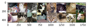
预测结果没有出现错误,但是还有进一步改进所的空间(本文输入时采用了随机裁剪,如果对原始图片进行缩放可能也会提升模型的预测准确率,还有增加训练次数和数据增强处理)。
完整代码链接:JaimeTang/PyTorch-and-TransferLearning
小结:
迁移学习的方法有快速解决同类问题的优点,类似问题不用再从头到尾对模型参数进行优化和训练。复杂模型的参数训练优化可能需要数周的时间,所以这个思路大大节约了时间成本。如果对模型训练结果不理想,还可以冻结更少分层次,训练更多的层次,而不是盲目的一开始便从头训练。也许正是这些优点也决定了迁移学习在实际中得到广泛应用的原因。
