In early 2015, Uber Engineering migrated its business entities from integer identifiers to UUID identifiers as part of an initiative towards using multiple active data centers. To achieve this, our Data Warehouse team was tasked with identifying every foreign-key relationship between every table in the data warehouse to backfill all the ID columns with corresponding UUIDs.¹
Given the decentralized ownership of our tables, this was not a simple endeavor. The most promising solution was to crowdsource the information by scraping all the SQL queries submitted to the warehouse and observing which columns were joined together. To serve this need, we built and open sourced Queryparser, our tool for parsing and analyzing SQL queries.
In this article, we discuss our implementation of Queryparser, the variety of applications it unlocked, and some problems and limitations encountered along the way.
Implementation
Internally, Queryparser is deployed in a streaming architecture, as shown in Figure 1, below:
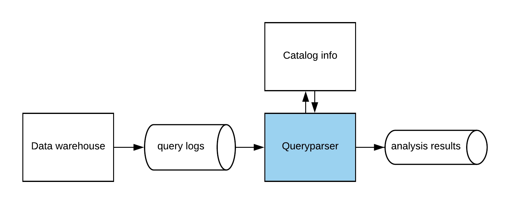
Figure 1: Uber’s data warehouse streaming architecture feeds all queries through Queryparser. Boxes denote services and pipes denote data-streams. The catalog info service is responsible for tracking the schemas of the tables in the data warehouse.
Queryparser consumes the real-time stream of queries submitted to the data warehouse, analyzes every single one, and emits the analysis results to a separate stream. Individual queries are processed in three steps, explained below and illustrated in Figure 2.
- Phase 1: Parse. Transforms the query from a raw string of characters into an abstract syntax tree (AST) representation.
- Phase 2: Resolve. Scans the raw AST and applies scoping rules. Transforms plain column names by adding the table name, and transforms plain table names by adding the schema name. Requires as input the full list of columns in every table and the full list of tables in every schema, otherwise known as “catalog information.”
- Phase 3: Analyze. Scans the resolved AST, looking for columns which are compared for equality.
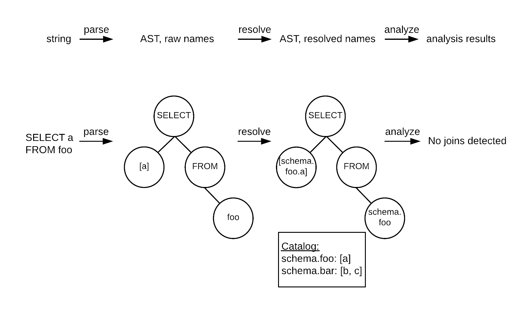
Figure 2: Queryparser takes three passes to fully process a query: parse, resolve, and analyze.The top flow illustrates this sequence conceptually as a transformation of data types. The bottom flow illustrates the sequence concretely on a real query.
The implementation and architecture successfully identified foreign-key relationships—a great result, given that the prototype only had partial coverage of the SQL grammar, the catalog information was entirely hard-coded, and our understanding of what counted as a foreign-key relationship was continually evolving.²
The Haskell choice
One of the first things you may have noticed in the open source Queryparser repository is that it is written in Haskell. Queryparser was originally conceived by an Uber engineer who was a Haskell enthusiast, and it quickly gained traction with several other engineers. In fact, many of us learned Haskell specifically to develop in it.
Haskell turned out to be a good choice for prototyping Queryparser for a variety of reasons. To start, Haskell has very mature library support for language parsers. Its expressive type system was also extremely useful for the frequent and extensive refactors of our internal model of a SQL query. Additionally, we leaned heavily on the compiler to guide us through those big, scary refactors. If we attempted the same using a dynamically-typed language, we would have lost weeks chasing runtime bugs that Haskell’s compiler can quickly flag for us.
The main drawback of writing Queryparser in Haskell was that not enough developers knew it. To introduce more of our engineers to Haskell, we started a weekly reading group, which met over lunch to discuss Haskell books and documentation.
Note that for interoperability with the rest of Uber’s non-Haskell infrastructure, Queryparser was (and is) deployed behind a Python proxy server. See the Deploying Queryparser section of this article for more details.
Diversity of solutions
After the initial success of Queryparser, we considered other ways in which the tool could improve our data warehouse operations. In addition to implementing join detection, we decided to implement several more analysis functions:
- Table access: which tables were accessed in the query
- Column access: which columns were accessed in each clause of the query
- Table lineage: which tables were modified by the query, and what were the inputs that determined their final state
Together, the new analyses gave a nuanced understanding of the access patterns in our data warehouse, permitting advances in the following areas: table administration, targeted communication, understanding data flow, incident response, and defensive operations, outlined below:
Table administration
As far as table administration was concerned, the benefits were threefold. First, table access statistics let us free up storage and compute resources by finding tables that were infrequently accessed and then removing them.
Second, column access statistics let us improve database performance by optimizing table layouts on disk, particularly with Vertica projections. The trick was to set the top GROUP BY columns as the shard keys and the top ORDER BY columns as the order keys.
Finally, column join statistics let us improve data usability and reduce database load by identifying clusters of tables that were frequently joined together and replacing them with a single dimensionally modeled table.
Targeted communication
Table access statistics let us send targeted communications to data consumers. Instead of blasting the entire Data Engineering mailing-list with updates about table schemas or data quality issues, we could notify only the data consumers who had recently accessed the table.
Understanding data flow
Table lineage data unlocked a special use case: if a sequence of queries were analyzed together, then the table lineage data could be aggregated to produce a graph of dataflow across the sequence.
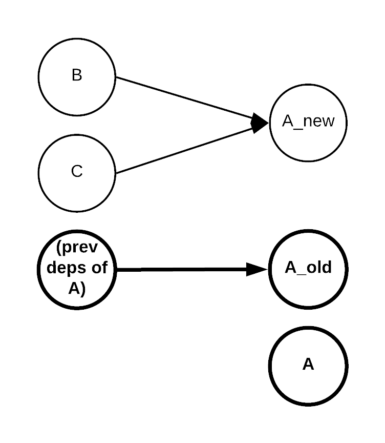
For example, consider the hypothetical SQL in Figure 3, below, which produces a new version of modeled table A from dependent tables B and C:
| Query |
| drop A_new if exists |
| create A_new as select … from B |
| insert into A_new select … from C |
| drop A_old if exists |
| rename A to A_old |
| rename A_new to A |
Figure 3: Sequence of SQL queries for computing modeled table A from dependent tables B and C.
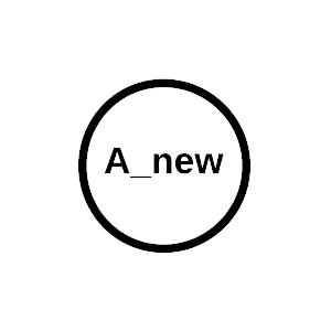
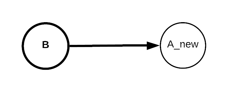
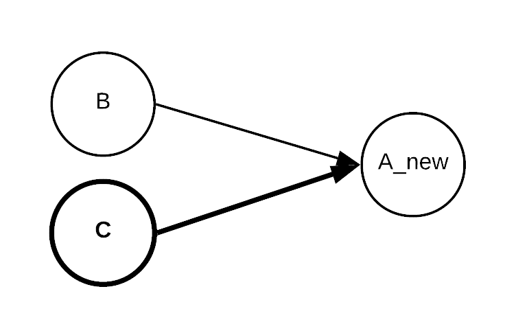
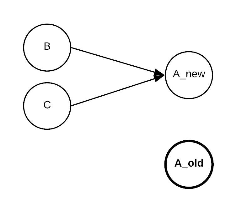
In Figure 4, below, we describe the table lineage that Queryparser would produce for each query in the sequence. Additionally, we depict and explain the cumulative observed dataflow for each query in the sequence. At the end, the cumulative data flow (correctly!) records that table A has dependencies on tables B and C:
Figure 4: SQL from Figure 3, with table lineage for each query in the sequence, and cumulative table lineage for the entire sequence.
We modified our ETL-framework to record the sequence of SQL queries in every ETL and submit them to Queryparser, at which point Queryparser was programmatically generating graphs of data-flow for all the modeled tables in our warehouse. See Figure 5, below, for an example:
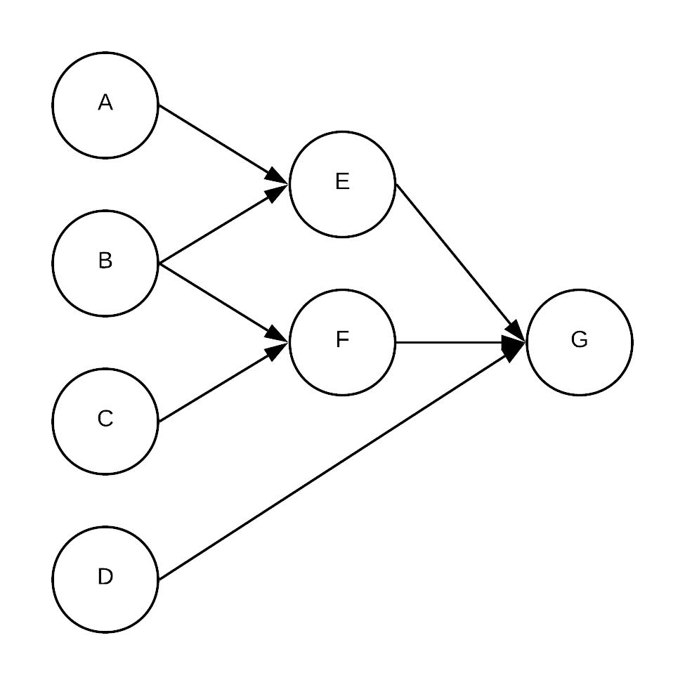
Figure 5: A sample data flow graph representing four raw tables (A, B, C, D) and three modeled tables (E, F, G) portrays how queries are processed by Queryparser. In practice, the raw tables typically come from upstream operational systems such as Kafka topics, Schemaless datastores, and service-oriented architecture (SOA) database tables. The modeled tables are exposed in the data warehouse (Hive) and in downstream data marts (Vertica).
Incident response
Table lineage data has been useful in responding to data quality incidents, decreasing the mitigation time by offering tactical visibility into incident impact. For example, given the table dependencies in Figure 5, if there was an issue in raw table A, we would know that the scope of impact included the modeled tables E and G. We would also know that once the issue was resolved, E and G would need to be backfilled. To address this, we could combine the lineage data with table access data to send targeted communications to all users of E and G.
Table lineage data is also useful for identifying the root cause of an incident. For instance, if there was an issue with modeled table E in Figure 5, it could only be due to the raw tables A or B. If there was an issue with modeled table G, it could be due to raw tables A, B, C, or D.
Defensive operations
Finally, the ability to analyze queries at runtime unlocked defensive operations tactics that enabled our data warehouse to run more smoothly. With Queryparser, queries can be intercepted en route to the data warehouse and submitted for analysis. If Queryparser detects parse errors or certain query anti-patterns, then the query can be rejected, reducing the overall load on the data warehouse.
Problems and limitations
Fred Brooks famously argued that there is no silver bullet in software engineering. While beneficial for our storage needs, Queryparser was no exception. As the project unfolded, it revealed some interesting essential complexities.
Long tail of language features
First, and least surprising: when adding support for a new SQL dialect, there is a long tail of infrequently-used language features to implement, which can require significant changes to Queryparser’s internal representation of a query. This was immediately apparent during the prototype phase, when Queryparser exclusively handled Vertica, and was further confirmed when support for Hive and Presto was added. For example, parsing TIMESERIES and OFFSET in Vertica required adding new clauses to SELECT statements. Additionally, parsing LEFT SEMI JOINs in Hive required a new join type with special scoping rules, and parsing the bonus top-level namespace of “databases” in Presto (where tables belong to schemas belong to databases) required extensive re-working of struct-access parsing.³
Tracking catalog state
Second, tracking catalog state was hard. Recall that catalog information is needed for resolving column names and table names. Uber’s data warehouse supports highly concurrent workloads, including concurrent schema changes, typically creating, dropping, and renaming tables, or adding or dropping columns from an existing table. We experimented briefly with using Queryparser to track catalog state; if Queryparser was already analyzing every query, we wondered if we could simply add an analysis that reported the schema changes and produce the new catalog state by applying them to the previous catalog state. Ultimately, that approach was unsuccessful due to the difficulty of ordering the entire stream of queries. Instead, our alternative (and more effective) approach was to treat the catalog state as more-or-less static, tracking the schema membership and column-lists of tables through configuration files.
Sessionizing queries
Third, sessionizing queries with Queryparser was difficult. In a perfect world, Queryparser would be able to track table lineage across an entire database session, accounting for transactions and rollbacks and various levels of transaction isolation. In practice, however, reconstructing database sessions from the query logs was difficult, so we decided not to add table lineage support for those features. Instead, Queryparser relies on Uber’s ETL-framework to sessionize the ETL queries on its behalf.
Leaky abstraction
Finally, Hive is a leaky abstraction over the underlying filesystem. For instance, INSERTs can be accomplished by several means:
- INSERT INTO foo SELECT … FROM bar
- ALTER TABLE foo ADD PARTITION … LOCATION ‘/hdfs/path/to/partition/in/bar’
Uber’s ETL framework initially used the first method, but was migrated to use the second method, as it showed dramatic performance improvements. This caused issues with table lineage data, as ‘/hdfs/path/to/partition/in/bar’ was not interpreted by Queryparser as corresponding to table bar. This particular issue was temporarily mitigated with a regular expression to infer the table name from the HDFS path. However, in general, if you choose to bypass the SQL abstractions of Hive in favor of filesystem-layer operations, then you opt out of Queryparser analysis.
Deploying Queryparser
Deploying a Haskell service in Uber’s non-Haskell infrastructure required some minor creativity, but never amounted to a substantial problem.
Installing Haskell itself was straightforward. Uber’s standard infrastructure pattern is to run every service in a Docker container. Container-level dependencies are managed through config files, so adding Haskell support was as simple as adding Stack to the list of required packages.
Queryparser is internally deployed as a Haskell artifact, running behind a Python service wrapper for interoperability with the rest of Uber’s infrastructure. The Python wrapper acts as a proxy server and simply forwards requests to the Haskell backend server in the same docker container. The Haskell server consists of a main thread that listens for requests on a UNIX-domain socket; when a new request arrives, the main thread spawns a worker thread to handle the request.
The Python wrapper also handles metric emission on behalf of the Haskell backend. Metric data is passed via a second UNIX-domain socket, with data flowing in the reverse direction: a daemon-thread in the Python layer listens for metrics from the Haskell layer.
In order to share configuration between the Python and Haskell layers, we implemented a tiny configuration parser in Haskell, which understood Uber’s standard Python convention of layered configuration files.
Finally, to define the service interface, we used Thrift. This is the standard choice at Uber, and since Thrift has Haskell support, the Haskell server worked out-of-the-box. Writing the Python code to transparently forward requests required diving into the binary protocol and was the most difficult operations step.
Summary
Queryparser unlocked a diversity of solutions and had some interesting limitations. From its humble origins as a migration tool, it became a vehicle for insight into large-scale data access patterns.
If you are interested in working on similar projects, reach out to za@uber.com and/or apply for a role on with us via the Uber Careers page and tell your Uber recruiter that you’d like to work on the Data Knowledge Platform team.
End Notes:
¹Spoiler alert: there ended up being dozens of primary keys to migrate. Each primary key could have many foreign keys under different aliases. The worst offender had over 50 different aliases.
² Foreign-key relationships ranged from the obvious like “SELECT * FROM foo JOIN bar ON foo.a = bar.b” to the less obvious like “SELECT * FROM foo WHERE foo.a IN (SELECT b from bar)” to the debatable like “SELECT a FROM foo UNION SELECT b FROM bar”. We erred on the side of being liberal about what we counted as a relationship, since output would be manually inspected anyway.
³ Given the SQL “w.x.y.z”, which identifier is the column name? Depending on the catalog state and what is in scope, it could be “w” with “x.y.z” referring to nested struct fields, or it could be “z” with “w.x.y” referring to “database.schema.table”, or anything in between.
