简介

实现任何程度或者级别的人工智能所必需的最大突破之一就是拥有可以处理文本数据的机器。值得庆幸的是，全世界文本数据的数量在最近几年已经实现指数级增长。这也迫切需要人们从文本数据中挖掘新知识、新观点。从社交媒体分析到风险管理和网络犯罪保护，处理文本数据已经变得前所未有的重要。

image

在这篇文章中，我们将要讨论不同的特征提取方法，从一些基本技巧逐步深入学习高级自然语言处理技术。我们也将会学习如何预处理文本数据，以便可以从“干净”数据中提取更好的特征。

1. 基本特征提取

即使我们对NLP没有充足的知识储备，但是我们可以使用python来提取文本数据的几个基本特征。在开始之前，我们使用pandas将数据集加载进来，以便后面其他任务的使用，数据集是Twitter情感文本数据集。

import pandas as pd
train=pd.read_csv("files/data/python46-data/train_E6oV3lV.csv")
print(train.head(10))

   id  label                                              tweet
0   1      0   @user when a father is dysfunctional and is s...
1   2      0  @user @user thanks for #lyft credit i can't us...
2   3      0                                bihday your majesty
3   4      0  #model   i love u take with u all the time in ...
4   5      0             factsguide: society now    #motivation
5   6      0  [2/2] huge fan fare and big talking before the...
6   7      0   @user camping tomorrow @user @user @user @use...
7   8      0  the next school year is the year for exams.ð��...
8   9      0  we won!!! love the land!!! #allin #cavs #champ...
9  10      0   @user @user welcome here !  i'm   it's so #gr...

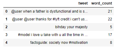
1.1 词汇数量

对每一条推文，我们可以提取的最基本特征之一就是词语数量。这样做的初衷就是通常情况下，负面情绪评论含有词语数量比正面情绪评论多。

我们可以简单地调用split函数，将句子切分：

train['word_count']=train['tweet'].apply(lambda x:len(str(x).split(" ")))
train[['tweet','word_count']].head()

1.2 字符数量

选择字符数量作为特征的原因和前一个特征一样。在这里，我们直接通过字符串长度计算每条推文字符数量

train['char_count']=train['tweet'].str.len()
train[['tweet','char_count']].head()

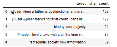
注意这里字符串的个数包含了推文中的空格个数，我们根据需要自行去除掉

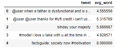
1.3 平均词汇长度

我们接下来将计算每条推文的平均词汇长度作为另一个特征，这个有可能帮助我们改善模型。将每条推文所有单词的长度然后除以每条推文单词的个数，即可作为平均词汇长度

def avg_word(sentence):
    words=sentence.split()
    return (sum(len(word) for word in words)/len(words))

train['avg_word']=train['tweet'].apply(lambda x:avg_word(x))
train[['tweet','avg_word']].head()

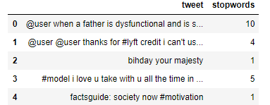
1.4 停用词的数量

通常情况下，在解决NLP问题时，首要任务时去除停用词（stopword）。但是有时计算停用词的数量可以提供我们之前失去的额外信息。下面关于停用词的解释：

为节省存储空间和提高搜索效率，搜索引擎在索引页面或处理搜索请求时会自动忽略某些字或词，这些字或词即被称为Stop Words(停用词)。通常意义上，Stop Words大致为如下两类：

这些词应用十分广泛，在Internet上随处可见，比如“Web”一词几乎在每个网站上均会出现，对这样的词搜索引擎无法保证能够给出真正相关的搜索结果，难以帮助缩小搜索范围，同时还会降低搜索的效率；
这类就更多了，包括了语气助词、副词、介词、连接词等，通常自身并无明确的意义，只有将其放入一个完整的句子中才有一定作用，如常见的“的”、“在”之类。

在这里，我们导入NLTK库中的stopwors模块

from nltk.corpus import stopwords
stop=stopwords.words('english')
train['stopwords']=train['tweet'].apply(lambda sen:len([x for x in sen.split() if x in stop]))
train[['tweet','stopwords']].head()

1.5 特殊字符的数量

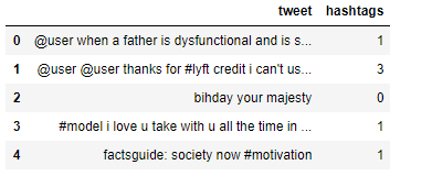
一个比较有趣的特征就是我们可以从每个推文中提取“#”和“@”符号的数量。这也有利于我们从文本数据中提取更多信息

这里我们使用startswith函数来处理

train['hashtags']=train['tweet'].apply(lambda sen:len([x for x in sen.split() if x.startswith("#")]))
train[['tweet','hashtags']].head()

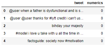
1.6 数字的数量

这个特征并不常用，但是在做相似任务时，数字数量是一个比较有用的特征

train['numerics']=train['tweet'].apply(lambda sen:len([x for x in sen.split() if x.isdigit()]))
train[['tweet','numerics']].head()

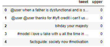
1.7 大写单词的数量

“Anger”或者 “Rage”通常情况下使用大写来表述，所以有必要去识别出这些词

train['upper']=train['tweet'].apply(lambda sen:len([x for x in sen.split() if x.isupper()]))
train[['tweet','upper']].head()

2 文本数据的预处理

到目前为止,我们已经学会了如何从文本数据中提取基本特征。深入文本和特征提取之前,我们的第一步应该是清洗数据,以获得更好的特性。

我们将实现这一目标做一些基本的训练数据预处理步骤。

2.1 小写转化

预处理的第一步,我们要做的是把我们的推文变成小写。这避免了拥有相同的多个副本。例如,当我们计算字词汇数量时,“Analytics”和“analytics”将被视为不同的单词。

train['tweet']=train['tweet'].apply(lambda sen:" ".join(x.lower() for x in sen.split()))
train['tweet'].head()

0    @user when a father is dysfunctional and is so...
1    @user @user thanks for #lyft credit i can't us...
2                                  bihday your majesty
3    #model i love u take with u all the time in ur...
4                  factsguide: society now #motivation
Name: tweet, dtype: object

2.2 去除标点符号

下一步是去除标点符号,因为它在文本数据中不添加任何额外的信息。因此删除的所有符号将帮助我们减少训练数据的大小。

train['tweet'] = train['tweet'].str.replace('[^\w\s]','')
train['tweet'].head()

0    user when a father is dysfunctional and is so ...
1    user user thanks for lyft credit i cant use ca...
2                                  bihday your majesty
3    model i love u take with u all the time in urð...
4                    factsguide society now motivation
Name: tweet, dtype: object

正如你所看到的在上面的输出中,所有的标点符号,包括"#"和"@"已经从训练数据中去除

2.3 停用词去除

正如我们前面所讨论的,停止词(或常见单词)应该从文本数据中删除。为了这个目的,我们可以创建一个列表stopwords作为自己停用词库或我们可以使用预定义的库。

from nltk.corpus import stopwords
stop=stopwords.words('english')
train['tweet']=train['tweet'].apply(lambda sen:" ".join(x for x in sen.split() if x not in stop))
train['tweet'].head()

0    user father dysfunctional selfish drags kids d...
1    user user thanks lyft credit cant use cause do...
2                                       bihday majesty
3                model love u take u time urð ðððð ððð
4                        factsguide society motivation
Name: tweet, dtype: object

2.4 常见词去除

我们可以把常见的单词从文本数据首先,让我们来检查中最常出现的10个字文本数据然后再调用删除或保留。

freq=pd.Series(' '.join(train['tweet']).split()).value_counts()[:10]
freq

user     17473
love      2647
ð         2511
day       2199
â         1797
happy     1663
amp       1582
im        1139
u         1136
time      1110
dtype: int64

现在我们把这些词去除掉，因为它们对我们文本数据分类没有任何作用

freq=list(freq.index)
freq

['user', 'love', 'ð', 'day', 'â', 'happy', 'amp', 'im', 'u', 'time']

train['tweet']=train['tweet'].apply(lambda sen:' '.join(x for x in sen.split() if x not in freq))
train['tweet'].head()

0    father dysfunctional selfish drags kids dysfun...
1    thanks lyft credit cant use cause dont offer w...
2                                       bihday majesty
3                              model take urð ðððð ððð
4                        factsguide society motivation
Name: tweet, dtype: object

2.5 稀缺词去除

同样,正如我们删除最常见的话说,这一次让我们从文本中删除很少出现的词。因为它们很稀有,它们之间的联系和其他词主要是噪音。可以替换罕见的单词更一般的形式,然后这将有更高的计数。

freq = pd.Series(' '.join(train['tweet']).split()).value_counts()[-10:]
freq

happenedâ       1
britmumspics    1
laterr          1
2230            1
dkweddking      1
ampsize         1
moviescenes     1
kaderimsin      1
nfinity         1
babynash        1
dtype: int64

freq = list(freq.index)
train['tweet'] = train['tweet'].apply(lambda x: " ".join(x for x in x.split() if x not in freq))
train['tweet'].head()

0    father dysfunctional selfish drags kids dysfun...
1    thanks lyft credit cant use cause dont offer w...
2                                       bihday majesty
3                              model take urð ðððð ððð
4                        factsguide society motivation
Name: tweet, dtype: object

所有这些预处理步骤是必不可少的,帮助我们减少我们的词汇噪音,这样最终产生更有效的特征。

2.6 拼写校对

我们都见过推文存在大量的拼写错误。我们再短时间内匆忙发送tweet,很难发现这些错误。在这方面,拼写校正是一个有用的预处理步骤,因为这也会帮助我们减少单词的多个副本。例如,“Analytics”和“analytcs”将被视为不同的单词,即使它们在同一意义上使用。

为实现这一目标,我们将使用textblob库。

TextBlob是一个用Python编写的开源的文本处理库。它可以用来执行很多自然语言处理的任务，比如，词性标注，名词性成分提取，情感分析，文本翻译，等等。你可以在官方文档阅读TextBlog的所有特性。

from textblob import TextBlob
train['tweet'][:5].apply(lambda x: str(TextBlob(x).correct()))

0    father dysfunctional selfish drags kiss dysfun...
1    thanks left credit can use cause dont offer wh...
2                                       midday majesty
3                               model take or ðððð ððð
4                        factsguide society motivation
Name: tweet, dtype: object

注意,它会花费很多时间去做这些修正。因此,为了学习的目的,我只显示这种技术运用在前5行的效果。

另外在使用这个技术之前，需要小心一些，因为如果推文中存在大量缩写，比如“your”缩写为“ur”，那么将修正为“or”

2.7 分词

分词是指将文本划分为一系列的单词或词语。在我们的示例中,我们使用了textblob库

TextBlob(train['tweet'][1]).words

WordList(['thanks', 'lyft', 'credit', 'cant', 'use', 'cause', 'dont', 'offer', 'wheelchair', 'vans', 'pdx', 'disapointed', 'getthanked'])

2.8 词干提取

词形还原（lemmatization），是把一个任何形式的语言词汇还原为一般形式（能表达完整语义），而词干提取
（stemming）是抽取词的词干或词根形式（不一定能够表达完整语义）。词形还原和词干提取是词形规范化的两类重要方式，都能够达到有效归并词形的目的，二者既有联系也有区别。具体介绍请参考词干提取（stemming）和词形还原（lemmatization）

词干提取(stemming)是指通过基于规则的方法去除单词的后缀，比如“ing”,“ly”，“s”等等。

from nltk.stem import PorterStemmer
st=PorterStemmer()
train['tweet'][:5].apply(lambda x:" ".join([st.stem(word) for word in x.split()]))

0        father dysfunct selfish drag kid dysfunct run
1    thank lyft credit cant use caus dont offer whe...
2                                       bihday majesti
3                              model take urð ðððð ððð
4                              factsguid societi motiv
Name: tweet, dtype: object

在上面的输出中，“dysfunctional ”已经变为“dysfunct ”

2.9 词性还原

词形还原处理后获得的结果是具有一定意义的、完整的词，一般为词典中的有效词

from textblob import Word
train['tweet']=train['tweet'].apply(lambda x:" ".join([Word(word).lemmatize() for word in x.split()]))
train['tweet'].head()

0    father dysfunctional selfish drag kid dysfunct...
1    thanks lyft credit cant use cause dont offer w...
2                                       bihday majesty
3                              model take urð ðððð ððð
4                        factsguide society motivation
Name: tweet, dtype: object

3 高级文本处理

到目前为止,我们已经做了所有的可以清洗我们数据的预处理基本步骤。现在,我们可以继续使用NLP技术提取特征。

3.1 N-grams

N-grams称为N元语言模型，是多个词语的组合，是一种统计语言模型，用来根据前(n-1)个item来预测第n个item。常见模型有一元语言模型(unigrams)、二元语言模型（bigrams ）、三元语言模型(trigrams )。

Unigrams包含的信息通常情况下比bigrams和trigrams少，需要根据具体应用选择语言模型，因为如果n-grams太短，这时不能捕获重要信息。另一方面，如果n-grams太长，那么捕获的信息基本上是一样的，没有差异性

TextBlob(train['tweet'][0]).ngrams(2)

[WordList(['father', 'dysfunctional']),
 WordList(['dysfunctional', 'selfish']),
 WordList(['selfish', 'drag']),
 WordList(['drag', 'kid']),
 WordList(['kid', 'dysfunction']),
 WordList(['dysfunction', 'run'])]

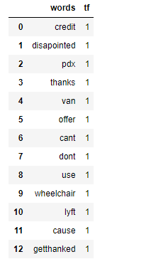
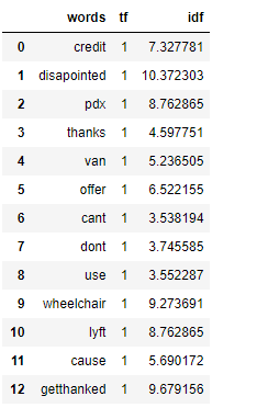
3.2 词频

词频(Term frequency)就是一个单词在一个句子出现的次数与这个句子单词个数的比例。

** TF = (Number of times term T appears in the particular row) / (number of terms in that row)**

tf1 = (train['tweet'][1:2]).apply(lambda x: pd.value_counts(x.split(" "))).sum(axis = 0).reset_index()
tf1.columns = ['words','tf']
tf1

3.3 反转文档频率

反转文档频率(Inverse Document Frequency)，简称为IDF，其原理可以简单理解为如果一个单词在所有文档都会出现，那么可能这个单词对我们没有那么重要。

一个单词的IDF就是所有行数与出现该单词的行的个数的比例，最后对数。
IDF = log(N/n)

import numpy as np
for i,word in enumerate(tf1['words']):
    tf1.loc[i, 'idf'] =np.log(train.shape[0]/(len(train[train['tweet'].str.contains(word)])))
tf1

3.4 词频-反转文档频率(TF-IDF)

TF-IDF=TF*IDF

tf1['tfidf']=tf1['tf']*tf1['idf']
tf1

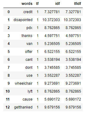
我们可以看到，TF-IDF已经“惩罚了”‘don’t’, ‘can’t’, 和‘use’,因为它们是通用词，tf-idf的值都比较低。

另外可以通过sksklearn直接计算tf-idf值

from sklearn.feature_extraction.text import TfidfVectorizer
tfidf = TfidfVectorizer(max_features=1000, lowercase=True, analyzer='word',
 stop_words= 'english',ngram_range=(1,1))
train_vect = tfidf.fit_transform(train['tweet'])

train_vect

<31962x1000 sparse matrix of type '<class 'numpy.float64'>'
    with 114055 stored elements in Compressed Sparse Row format>

3.5 词袋

BOW，就是将文本/Query看作是一系列词的集合。由于词很多，所以咱们就用袋子把它们装起来，简称词袋。至于为什么用袋子而不用筐（basket）或者桶（bucket），这咱就不知道了。举个例子：

               文本1：苏宁易购/是/国内/著名/的/B2C/电商/之一

这是一个短文本。“/”作为词与词之间的分割。从中我们可以看到这个文本包含“苏宁易购”，“B2C”，“电商”等词。换句话说，该文本的的词袋由“苏宁易购”，“电商”等词构成。

详细请参考词袋模型和词向量模型

from sklearn.feature_extraction.text import CountVectorizer
bow = CountVectorizer(max_features=1000, lowercase=True, ngram_range=(1,1),analyzer = "word")
train_bow = bow.fit_transform(train['tweet'])
train_bow

<31962x1000 sparse matrix of type '<class 'numpy.int64'>'
    with 128402 stored elements in Compressed Sparse Row format>

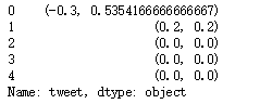
3.6 情感分析

我们最终需要解决的任务就是如何对推文进行情感分析，在使用ML/DL模型之前，我们可以使用textblob库去进行评测情感

train['tweet'][:5].apply(lambda x:TextBlob(x).sentiment)

0    (-0.3, 0.5354166666666667)
1                    (0.2, 0.2)
2                    (0.0, 0.0)
3                    (0.0, 0.0)
4                    (0.0, 0.0)
Name: tweet, dtype: object

使用TextBlob情感分析的结果，以元组的方式进行返回，形式如(polarity, subjectivity). 其中polarity的分数是一个范围为 [-1.0 , 1.0 ] 浮点数, 正数表示积极，负数表示消极。subjectivity 是一个范围为 [0.0 , 1.0 ] 的浮点数，其中 0.0 表示客观，1.0表示主观的。

下面是一个简单实例

from textblob import TextBlob
testimonial = TextBlob("Textblob is amazingly simple to use. What great fun!")
print(testimonial.sentiment)

Sentiment(polarity=0.39166666666666666, subjectivity=0.4357142857142857)

train['sentiment'] = train['tweet'].apply(lambda x: TextBlob(x).sentiment[0] )
train[['id','tweet','sentiment']].head()

4.7 词嵌入

词嵌入就是文本的向量化表示，潜在思想就是相似单词的向量之间的距离比较短。

from gensim.scripts.glove2word2vec import glove2word2vec
glove_input_file = 'glove.6B.100d.txt'
word2vec_output_file = 'glove.6B.100d.txt.word2vec'
glove2word2vec(glove_input_file, word2vec_output_file)

总结

通过这篇文章，希望大家对文本数据处理步骤以及特征选择有了大致了解，推荐大家在这些基础之上，使用机器学习或者深度学习方法进行情感预测

文章来自于www.analyticsvidhya.com/blog/2017/0…

文本数据处理的终极指南-[NLP入门]

简介

目录