根据股票历史数据中的最低价、最高价、开盘价、收盘价、交易量、交易额、跌涨幅等因素，对下一日股票最高价进行预测。

实验用到的数据长这个样子：

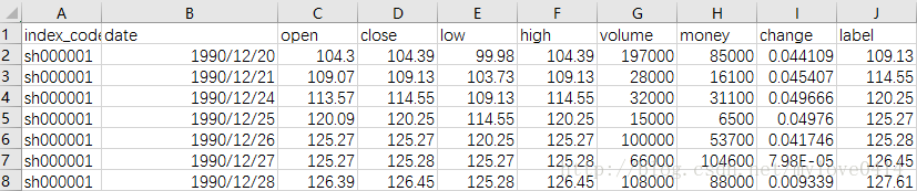
label是标签y，也就是下一日的最高价。列C——I为输入特征。 本实例用前5800个数据做训练数据。

单因素输入特征及RNN、LSTM的介绍请戳上一篇 Tensorflow实例：利用LSTM预测股票每日最高价（一）

导入包及声明常量

import pandas as pd
import numpy as np
import tensorflow as tf

#定义常量
rnn_unit=10       #hidden layer units
input_size=7      
output_size=1
lr=0.0006         #学习率

导入数据

f=open('dataset.csv') 
df=pd.read_csv(f)     #读入股票数据
data=df.iloc[:,2:10].values   #取第3-10列

生成训练集、测试集

考虑到真实的训练环境，这里把每批次训练样本数（batch_size）、时间步（time_step）、训练集的数量（train_begin,train_end）设定为参数，使得训练更加机动。

#——————————获取训练集——————————
def get_train_data(batch_size=60,time_step=20,train_begin=0,train_end=5800):
    batch_index=[]
    data_train=data[train_begin:train_end]
    normalized_train_data=(data_train-np.mean(data_train,axis=0))/np.std(data_train,axis=0)  #标准化
    train_x,train_y=[],[]   #训练集x和y初定义
    for i in range(len(normalized_train_data)-time_step):
       if i % batch_size==0:
           batch_index.append(i)
       x=normalized_train_data[i:i+time_step,:7]
       y=normalized_train_data[i:i+time_step,7,np.newaxis]
       train_x.append(x.tolist())
       train_y.append(y.tolist())
    batch_index.append((len(normalized_train_data)-time_step))
    return batch_index,train_x,train_y

#——————————获取测试集——————————
def get_test_data(time_step=20,test_begin=5800):
    data_test=data[test_begin:]
    mean=np.mean(data_test,axis=0)
    std=np.std(data_test,axis=0)
    normalized_test_data=(data_test-mean)/std  #标准化
    size=(len(normalized_test_data)+time_step-1)//time_step  #有size个sample 
    test_x,test_y=[],[]  
    for i in range(size-1):
       x=normalized_test_data[i*time_step:(i+1)*time_step,:7]
       y=normalized_test_data[i*time_step:(i+1)*time_step,7]
       test_x.append(x.tolist())
       test_y.extend(y)
    test_x.append((normalized_test_data[(i+1)*time_step:,:7]).tolist())
    test_y.extend((normalized_test_data[(i+1)*time_step:,7]).tolist())
    return mean,std,test_x,test_y

构建神经网络

#——————————————————定义神经网络变量——————————————————
def lstm(X):     
    batch_size=tf.shape(X)[0]
    time_step=tf.shape(X)[1]
    w_in=weights['in']
    b_in=biases['in']  
    input=tf.reshape(X,[-1,input_size])  #需要将tensor转成2维进行计算，计算后的结果作为隐藏层的输入
    input_rnn=tf.matmul(input,w_in)+b_in
    input_rnn=tf.reshape(input_rnn,[-1,time_step,rnn_unit])  #将tensor转成3维，作为lstm cell的输入
    cell=tf.nn.rnn_cell.BasicLSTMCell(rnn_unit)
    init_state=cell.zero_state(batch_size,dtype=tf.float32)
    output_rnn,final_states=tf.nn.dynamic_rnn(cell, input_rnn,initial_state=init_state, dtype=tf.float32)  #output_rnn是记录lstm每个输出节点的结果，final_states是最后一个cell的结果
    output=tf.reshape(output_rnn,[-1,rnn_unit]) #作为输出层的输入
    w_out=weights['out']
    b_out=biases['out']
    pred=tf.matmul(output,w_out)+b_out
    return pred,final_states

训练模型

#——————————————————训练模型——————————————————
def train_lstm(batch_size=80,time_step=15,train_begin=0,train_end=5800):
    X=tf.placeholder(tf.float32, shape=[None,time_step,input_size])
    Y=tf.placeholder(tf.float32, shape=[None,time_step,output_size])
    batch_index,train_x,train_y=get_train_data(batch_size,time_step,train_begin,train_end)
    pred,_=lstm(X)
    #损失函数
    loss=tf.reduce_mean(tf.square(tf.reshape(pred,[-1])-tf.reshape(Y, [-1])))
    train_op=tf.train.AdamOptimizer(lr).minimize(loss)
    saver=tf.train.Saver(tf.global_variables(),max_to_keep=15)
    module_file = tf.train.latest_checkpoint()    
    with tf.Session() as sess:
        #sess.run(tf.global_variables_initializer())
        saver.restore(sess, module_file)
        #重复训练2000次
        for i in range(2000):
            for step in range(len(batch_index)-1):
                _,loss_=sess.run([train_op,loss],feed_dict={X:train_x[batch_index[step]:batch_index[step+1]],Y:train_y[batch_index[step]:batch_index[step+1]]})
            print(i,loss_)
            if i % 200==0:
                print("保存模型：",saver.save(sess,'stock2.model',global_step=i))

嗯，这里说明一下，这里的参数是基于已有模型恢复的参数，意思就是说之前训练过模型，保存过神经网络的参数，现在再取出来作为初始化参数接着训练。如果是第一次训练，就用sess.run(tf.global_variables_initializer())，也就不要用到 module_file = tf.train.latest_checkpoint() 和saver.store(sess, module_file)了。

测试

#————————————————预测模型————————————————————
def prediction(time_step=20):
    X=tf.placeholder(tf.float32, shape=[None,time_step,input_size])
    mean,std,test_x,test_y=get_test_data(time_step)
    pred,_=lstm(X)     
    saver=tf.train.Saver(tf.global_variables())
    with tf.Session() as sess:
        #参数恢复
        module_file = tf.train.latest_checkpoint()
        saver.restore(sess, module_file) 
        test_predict=[]
        for step in range(len(test_x)-1):
          prob=sess.run(pred,feed_dict={X:[test_x[step]]})   
          predict=prob.reshape((-1))
          test_predict.extend(predict)
        test_y=np.array(test_y)*std[7]+mean[7]
        test_predict=np.array(test_predict)*std[7]+mean[7]
        acc=np.average(np.abs(test_predict-test_y[:len(test_predict)])/test_y[:len(test_predict)]) #acc为测试集偏差

最后的结果画出来是这个样子：

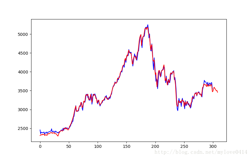
红色折线是真实值，蓝色折线是预测值

偏差大概在1.36%

代码和数据上传到了github上，想要的戳全部代码

注！：如要转载，请经过本人允许并注明出处！