Attention是一种用于提升基于RNN（LSTM或GRU）的Encoder + Decoder模型的效果的的机制（Mechanism），一般称为Attention Mechanism。Attention Mechanism目前非常流行，广泛应用于机器翻译、语音识别、图像标注（Image Caption）等很多领域，之所以它这么受欢迎，是因为Attention给模型赋予了区分辨别的能力，例如，在机器翻译、语音识别应用中，为句子中的每个词赋予不同的权重，使神经网络模型的学习变得更加灵活（soft），同时Attention本身可以做为一种对齐关系，解释翻译输入/输出句子之间的对齐关系，解释模型到底学到了什么知识，为我们打开深度学习的黑箱，提供了一个窗口。

我为大家收集的有关注意力机制的精华文章

标题	说明	附加
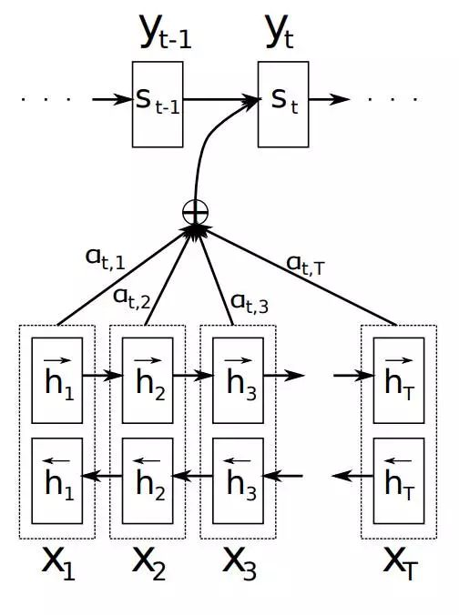
模型汇总24 - 深度学习中Attention Mechanism详细介绍：原理、分类及应用	首推知乎	2017
目前主流的attention方法都有哪些？	attention机制详解知乎	2017
Attention_Network_With_Keras 注意力模型的代码的实现与分析	代码解析简书	20180617
Attention_Network_With_Keras	代码实现 GitHub	2018
各种注意力机制窥探深度学习在NLP中的神威	综述机器之心	20181008

觉得不想看太多文字直接拖到文末看我的代码讲解，来个醍醐灌顶

以2014《Learning Phrase Representations using RNN Encoder-Decoder for Statistical Machine Translation》抛砖引玉

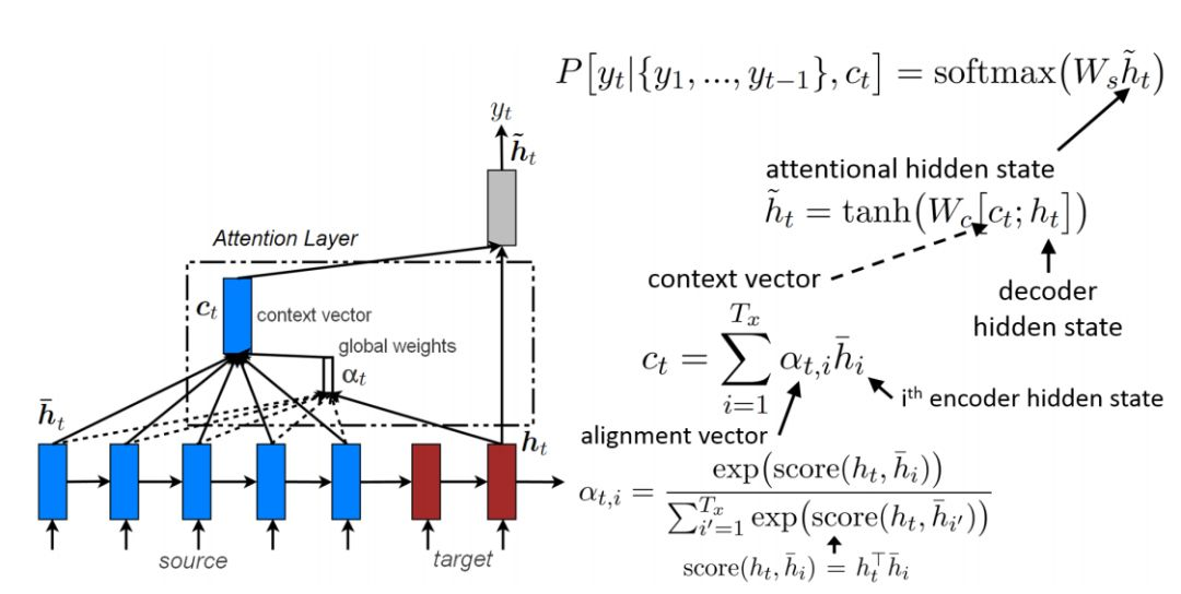
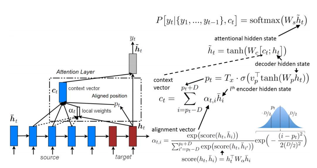
要介绍Attention Mechanism结构和原理，首先需要介绍下Seq2Seq模型的结构。基于RNN的Seq2Seq模型主要由两篇论文介绍，只是采用了不同的RNN模型。Ilya Sutskever等人与2014年在论文《Sequence to Sequence Learning with Neural Networks》中使用LSTM来搭建Seq2Seq模型。随后，2015年，Kyunghyun Cho等人在论文《Learning Phrase Representations using RNN Encoder–Decoder for Statistical Machine Translation》提出了基于GRU的Seq2Seq模型。两篇文章所提出的Seq2Seq模型，想要解决的主要问题是，如何把机器翻译中，变长的输入X映射到一个变长输出Y的问题，其主要结构如图所示。

传统的Seq2Seq结构

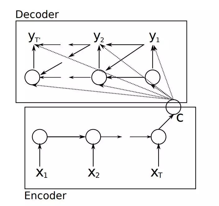
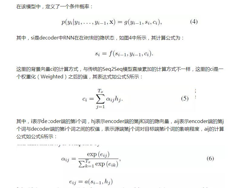
其中，Encoder把一个变成的输入序列x1，x2，x3....xt编码成一个固定长度隐向量（背景向量，或上下文向量context）c，c有两个作用：1、做为初始向量初始化Decoder的模型，做为decoder模型预测y1的初始向量。2、做为背景向量，指导y序列中每一个step的y的产出。Decoder主要基于背景向量c和上一步的输出yt-1解码得到该时刻t的输出yt，直到碰到结束标志（ $<EOS>$ ）为止。

如上文所述，传统的Seq2Seq模型对输入序列X缺乏区分度，因此，2015年，Kyunghyun Cho等人在论文《Learning Phrase Representations using RNN Encoder–Decoder for Statistical Machine Translation》中，引入了Attention Mechanism来解决这个问题，他们提出的模型结构如图所示。

Attention Mechanism模块图解

以Attention_Network_With_Keras 为例讲解一种Attention实现代码

部分代码

Tx = 50 # Max x sequence length
Ty = 5 # y sequence length
X, Y, Xoh, Yoh = preprocess_data(dataset, human_vocab, machine_vocab, Tx, Ty)

# Split data 80-20 between training and test
train_size = int(0.8*m)
Xoh_train = Xoh[:train_size]
Yoh_train = Yoh[:train_size]
Xoh_test = Xoh[train_size:]
Yoh_test = Yoh[train_size:]

To be careful, let's check that the code works:

i = 5
print("Input data point " + str(i) + ".")
print("")
print("The data input is: " + str(dataset[i][0]))
print("The data output is: " + str(dataset[i][1]))
print("")
print("The tokenized input is:" + str(X[i]))
print("The tokenized output is: " + str(Y[i]))
print("")
print("The one-hot input is:", Xoh[i])
print("The one-hot output is:", Yoh[i])

Input data point 5.

The data input is: 23 min after 20 p.m.
The data output is: 20:23

The tokenized input is:[ 5  6  0 25 22 26  0 14 19 32 18 30  0  5  3  0 28  2 25  2 40 40 40 40
 40 40 40 40 40 40 40 40 40 40 40 40 40 40 40 40 40 40 40 40 40 40 40 40
 40 40]
The tokenized output is: [ 2  0 10  2  3]

The one-hot input is: [[0. 0. 0. ... 0. 0. 0.]
 [0. 0. 0. ... 0. 0. 0.]
 [1. 0. 0. ... 0. 0. 0.]
 ...
 [0. 0. 0. ... 0. 0. 1.]
 [0. 0. 0. ... 0. 0. 1.]
 [0. 0. 0. ... 0. 0. 1.]]
The one-hot output is: [[0. 0. 1. 0. 0. 0. 0. 0. 0. 0. 0.]
 [1. 0. 0. 0. 0. 0. 0. 0. 0. 0. 0.]
 [0. 0. 0. 0. 0. 0. 0. 0. 0. 0. 1.]
 [0. 0. 1. 0. 0. 0. 0. 0. 0. 0. 0.]
 [0. 0. 0. 1. 0. 0. 0. 0. 0. 0. 0.]]

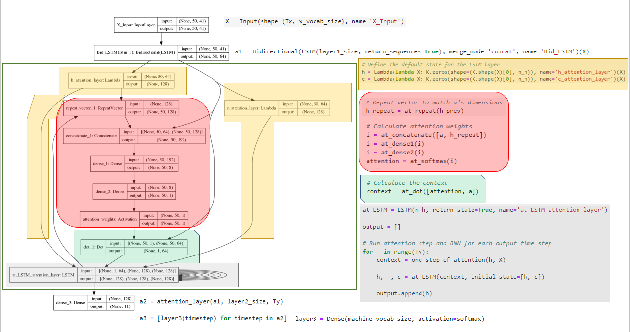
Model

Our next goal is to define our model. The important part will be defining the attention mechanism and then making sure to apply that correctly.

Define some model metadata:

layer1_size = 32
layer2_size = 128 # Attention layer

The next two code snippets defined the attention mechanism. This is split into two arcs:

Calculating context
Creating an attention layer

As a refresher, an attention network pays attention to certain parts of the input at each output time step. attention denotes which inputs are most relevant to the current output step. An input step will have attention weight ~1 if it is relevant, and ~0 otherwise. The context is the "summary of the input".

The requirements are thus. The attention matrix should have shape $(T_x)$ and sum to 1. Additionally, the context should be calculated in the same manner for each time step. Beyond that, there is some flexibility. This notebook calculates both this way:

attention = Softmax(Dense(Dense(x, y_{t-1})))

? context = \sum_{i=1}^{m} ( attention_i * x_i ) ?

For safety, $y_0$ is defined as $\vec{0}$ .

# Define part of the attention layer gloablly so as to
# share the same layers for each attention step.
def softmax(x):
    return K.softmax(x, axis=1)

at_repeat = RepeatVector(Tx)
at_concatenate = Concatenate(axis=-1)
at_dense1 = Dense(8, activation="tanh")
at_dense2 = Dense(1, activation="relu")
at_softmax = Activation(softmax, name='attention_weights')
at_dot = Dot(axes=1)

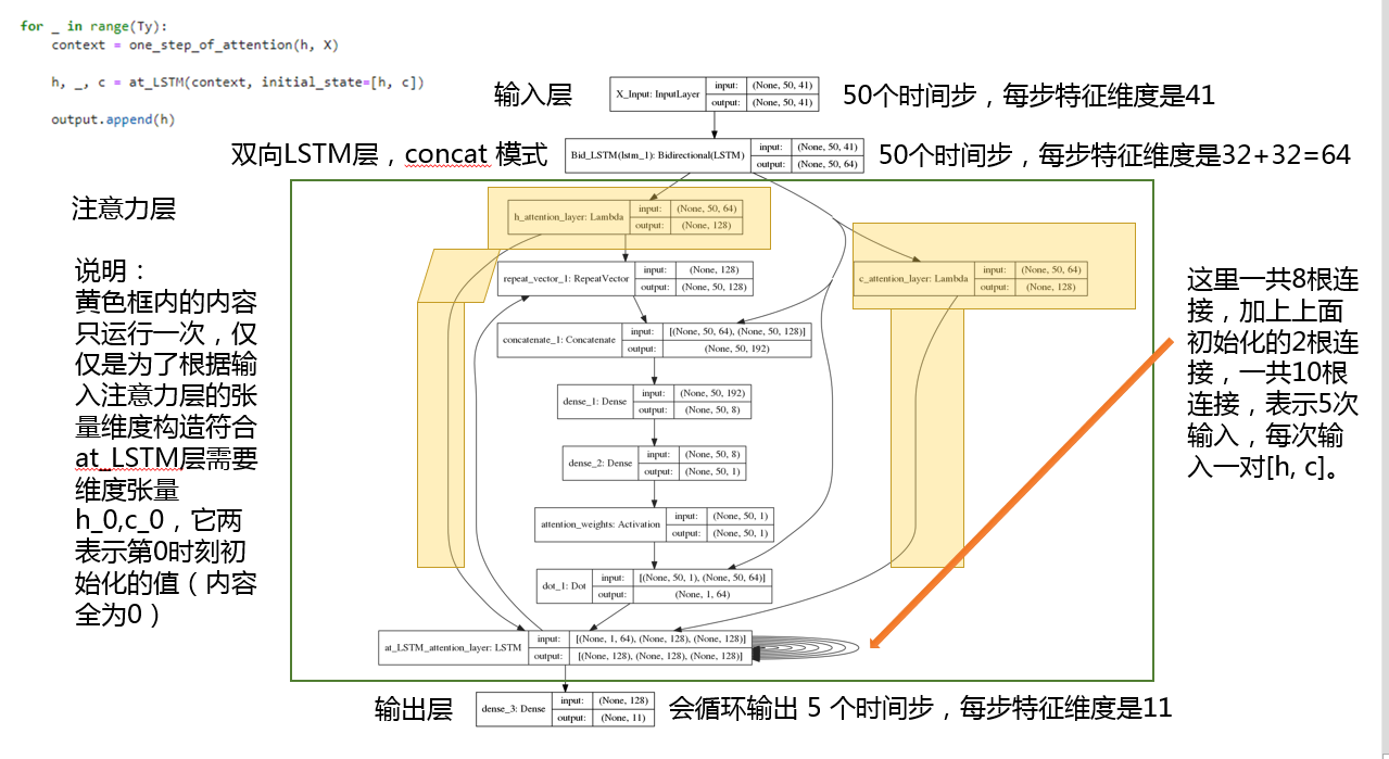
def one_step_of_attention(h_prev, a):
    """
    Get the context.

    Input:
    h_prev - Previous hidden state of a RNN layer (m, n_h)
    a - Input data, possibly processed (m, Tx, n_a)

    Output:
    context - Current context (m, Tx, n_a)
    """
    # Repeat vector to match a's dimensions
    h_repeat = at_repeat(h_prev)
    # Calculate attention weights
    i = at_concatenate([a, h_repeat])
    i = at_dense1(i)
    i = at_dense2(i)
    attention = at_softmax(i)
    # Calculate the context
    context = at_dot([attention, a])

    return context

def attention_layer(X, n_h, Ty):
    """
    Creates an attention layer.

    Input:
    X - Layer input (m, Tx, x_vocab_size)
    n_h - Size of LSTM hidden layer
    Ty - Timesteps in output sequence

    Output:
    output - The output of the attention layer (m, Tx, n_h)
    """    
    # Define the default state for the LSTM layer
    h = Lambda(lambda X: K.zeros(shape=(K.shape(X)[0], n_h)), name='h_attention_layer')(X)
    c = Lambda(lambda X: K.zeros(shape=(K.shape(X)[0], n_h)), name='c_attention_layer')(X)
    # Messy, but the alternative is using more Input()

    at_LSTM = LSTM(n_h, return_state=True, name='at_LSTM_attention_layer')

    output = []

    # Run attention step and RNN for each output time step
    for _ in range(Ty):
        context = one_step_of_attention(h, X)

        h, _, c = at_LSTM(context, initial_state=[h, c])

        output.append(h)

    return output

The sample model is organized as follows:

BiLSTM
Attention Layer
- Outputs Ty lists of activations.
Dense
- Necessary to convert attention layer's output to the correct y dimensions

layer3 = Dense(machine_vocab_size, activation=softmax)

def get_model(Tx, Ty, layer1_size, layer2_size, x_vocab_size, y_vocab_size):
    """
    Creates a model.

    input:
    Tx - Number of x timesteps
    Ty - Number of y timesteps
    size_layer1 - Number of neurons in BiLSTM
    size_layer2 - Number of neurons in attention LSTM hidden layer
    x_vocab_size - Number of possible token types for x
    y_vocab_size - Number of possible token types for y

    Output:
    model - A Keras Model.
    """

    # Create layers one by one
    X = Input(shape=(Tx, x_vocab_size), name='X_Input')

    a1 = Bidirectional(LSTM(layer1_size, return_sequences=True), merge_mode='concat', name='Bid_LSTM')(X)

    a2 = attention_layer(a1, layer2_size, Ty)

    a3 = [layer3(timestep) for timestep in a2]

    # Create Keras model
    model = Model(inputs=[X], outputs=a3)

    return model

The steps from here on out are for creating the model and training it. Simple as that.

# Obtain a model instance
model = get_model(Tx, Ty, layer1_size, layer2_size, human_vocab_size, machine_vocab_size)

plot_model(model, to_file='Attention_tutorial_model_copy.png', show_shapes=True)

模型结构及说明（重点来了）

模型评估

Evaluation

The final training loss should be in the range of 0.02 to 0.5

The test loss should be at a similar level.

# Evaluate the test performance
outputs_test = list(Yoh_test.swapaxes(0,1))
score = model.evaluate(Xoh_test, outputs_test)
print('Test loss: ', score[0])

2000/2000 [==============================] - 2s 1ms/step
Test loss:  0.4966005325317383

Now that we've created this beautiful model, let's see how it does in action.

The below code finds a random example and runs it through our model.

# Let's visually check model output.
import random as random

i = random.randint(0, m)

def get_prediction(model, x):
    prediction = model.predict(x)
    max_prediction = [y.argmax() for y in prediction]
    str_prediction = "".join(ids_to_keys(max_prediction, machine_vocab))
    return (max_prediction, str_prediction)

max_prediction, str_prediction = get_prediction(model, Xoh[i:i+1])

print("Input: " + str(dataset[i][0]))
print("Tokenized: " + str(X[i]))
print("Prediction: " + str(max_prediction))
print("Prediction text: " + str(str_prediction))

Input: 13.09
Tokenized: [ 4  6  2  3 12 40 40 40 40 40 40 40 40 40 40 40 40 40 40 40 40 40 40 40
 40 40 40 40 40 40 40 40 40 40 40 40 40 40 40 40 40 40 40 40 40 40 40 40
 40 40]
Prediction: [1, 3, 10, 0, 9]
Prediction text: 13:09

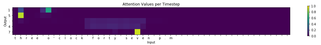
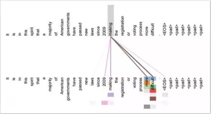
Last but not least, all introductions to Attention networks require a little tour.

The below graph shows what inputs the model was focusing on when writing each individual letter.

注意力机制图

注意力机制精要

全局注意力机制

局部注意力机制

自注意力机制

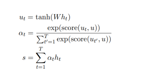
隐藏向量 $h_t$ 首先会传递到全连接层。然后校准系数 $a_t$ 会对比全连接层的输出 $u_t$ 和可训练上下文向量 u（随机初始化），并通过 Softmax 归一化而得出。注意力向量 s 最后可以为所有隐藏向量的加权和。上下文向量可以解释为在平均上表征的最优单词。但模型面临新的样本时，它会使用这一知识以决定哪一个词需要更加注意。在训练中，模型会通过反向传播更新上下文向量，即它会调整内部表征以确定最优词是什么。

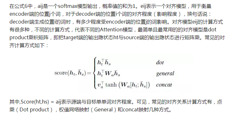
Self Attention与传统的Attention机制非常的不同：传统的Attention是基于source端和target端的隐变量（hidden state）计算Attention的，得到的结果是源端的每个词与目标端每个词之间的依赖关系。但Self Attention不同，它分别在source端和target端进行，仅与source input或者target input自身相关的Self Attention，捕捉source端或target端自身的词与词之间的依赖关系；然后再把source端的得到的self Attention加入到target端得到的Attention中，捕捉source端和target端词与词之间的依赖关系。因此，self Attention Attention比传统的Attention mechanism效果要好，主要原因之一是，传统的Attention机制忽略了源端或目标端句子中词与词之间的依赖关系，相对比，self Attention可以不仅可以得到源端与目标端词与词之间的依赖关系，同时还可以有效获取源端或目标端自身词与词之间的依赖关系

层级注意力机制

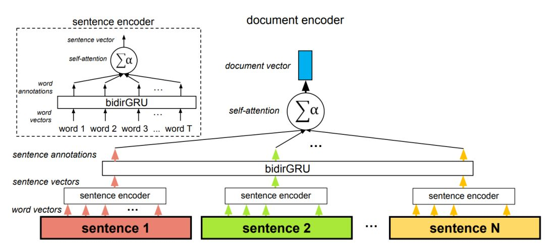
在该架构中，自注意力机制共使用了两次：在词层面与在句子层面。该方法因为两个原因而非常重要，首先是它匹配文档的自然层级结构（词——句子——文档）。其次在计算文档编码的过程中，它允许模型首先确定哪些单词在句子中是非常重要的，然后再确定哪个句子在文档中是非常重要的。

如果看完还是有疑惑或者想了解更多，请关注我博客望江人工智库，或者去 GitHub联系我。

关于注意力机制的实验，我完成之后会发布在我的 GitHub 上。

他们只说注意力机制（Attention Mechanism）不练，还是我来给大家撸代码讲解