

自本系列第一讲推出以来,得到了不少同学的反响和赞成,也有同学留言说最好能把数学推导部分写的详细点,笔者只能说尽力,因为打公式实在是太浪费时间了。。本节要和大家一起学习的是逻辑(logistic)回归模型,继续按照手推公式+纯 Python 的写作套路。
逻辑回归本质上跟逻辑这个词不是很搭边,叫这个名字完全是直译过来形成的。那该怎么叫呢?其实逻辑回归本名应该叫对数几率回归,是线性回归的一种推广,所以我们在统计学上也称之为广义线性模型。众多周知的是,线性回归针对的是标签为连续值的机器学习任务,那如果我们想用线性模型来做分类任何可行吗?答案当然是肯定的。
sigmoid 函数
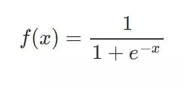
相较于线性回归的因变量 y 为连续值,逻辑回归的因变量则是一个 0/1 的二分类值,这就需要我们建立一种映射将原先的实值转化为 0/1 值。这时候就要请出我们熟悉的 sigmoid 函数了:
其函数图形如下:
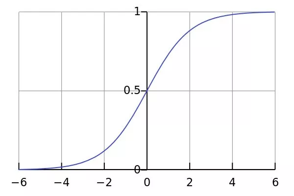
除了长的很优雅之外,sigmoid 函数还有一个很好的特性就是其求导计算等于下式,这给我们后续求交叉熵损失的梯度时提供了很大便利。

逻辑回归模型的数学推导
由 sigmoid 函数可知逻辑回归模型的基本形式为:

稍微对上式做一下转换:

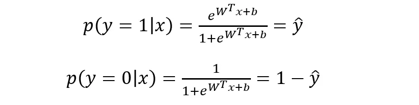
下面将 y 视为类后验概率 p(y = 1 | x),则上式可以写为:

则有:
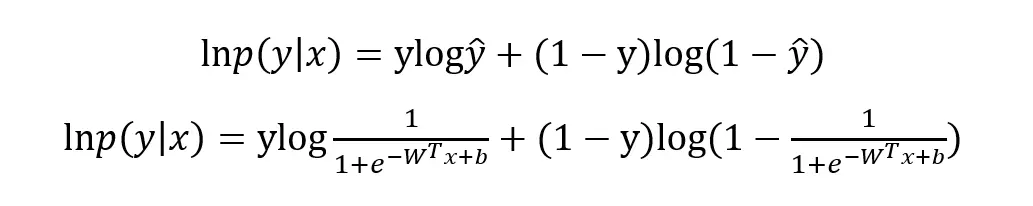
将上式进行简单综合,可写成如下形式:

写成对数形式就是我们熟知的交叉熵损失函数了,这也是交叉熵损失的推导由来:
最优化上式子本质上就是我们统计上所说的求其极大似然估计,可基于上式分别关于 W 和b 求其偏导可得:
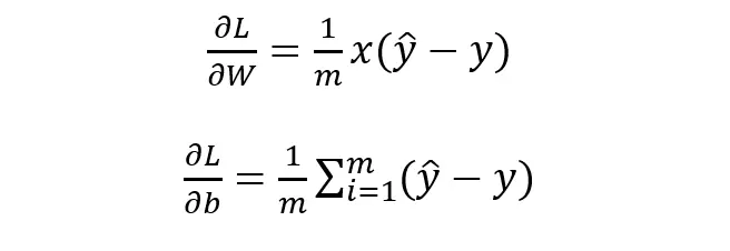
基于 W 和 b 的梯度进行权值更新即可求导参数的最优值,使得损失函数最小化,也即求得参数的极大似然估计,殊途同归啊。
逻辑回归的 Python 实现
跟上一讲写线性模型一样,在实际动手写之前我们需要理清楚思路。要写一个完整的逻辑回归模型我们需要:sigmoid函数、模型主体、参数初始化、基于梯度下降的参数更新训练、数据测试与可视化展示。
先定义一个 sigmoid 函数:
import numpy as np
def sigmoid(x):
    z = 1 / (1 + np.exp(-x))
    return z
定义模型参数初始化函数:
def initialize_params(dims):
    W = np.zeros((dims, 1))
    b = 0
    return W, b
定义逻辑回归模型主体部分,包括模型计算公式、损失函数和参数的梯度公式:
def logistic(X, y, W, b):
    num_train = X.shape[0]
    num_feature = X.shape[1]

    a = sigmoid(np.dot(X, W) + b)
    cost = -1/num_train * np.sum(y*np.log(a) + (1-y)*np.log(1-a))

    dW = np.dot(X.T, (a-y))/num_train
    db = np.sum(a-y)/num_train
    cost = np.squeeze(cost)

    return a, cost, dW, db
定义基于梯度下降的参数更新训练过程:
def logistic_train(X, y, learning_rate, epochs):
    # 初始化模型参数
    W, b = initialize_params(X.shape[1])
    cost_list = []

    # 迭代训练
    for i in range(epochs):
        # 计算当前次的模型计算结果、损失和参数梯度
        a, cost, dW, db = logistic(X, y, W, b)
        # 参数更新
        W = W -learning_rate * dW
        b = b -learning_rate * db

        # 记录损失
        if i % 100 == 0:
            cost_list.append(cost)
        # 打印训练过程中的损失
        if i % 100 == 0:
            print('epoch %d cost %f' % (i, cost))

    # 保存参数
    params = {
        'W': W,
        'b': b
    }
    # 保存梯度
    grads = {
        'dW': dW,
        'db': db
    }
    return cost_list, params, grads
定义对测试数据的预测函数:
def predict(X, params):
    y_prediction = sigmoid(np.dot(X, params['W']) + params['b'])
    for i in range(len(y_prediction)):
        if y_prediction[i] > 0.5:
            y_prediction[i] = 1
        else:
            y_prediction[i] = 0
    return y_prediction
使用 sklearn 生成模拟的二分类数据集进行模型训练和测试:
import matplotlib.pyplot as plt
from sklearn.datasets.samples_generator import make_classification
X,labels=make_classification(n_samples=100, n_features=2, n_redundant=0, n_informative=2, random_state=1, n_clusters_per_class=2)
rng=np.random.RandomState(2)
X+=2*rng.uniform(size=X.shape)
unique_lables=set(labels)
colors=plt.cm.Spectral(np.linspace(0, 1, len(unique_lables)))
for k, col in zip(unique_lables, colors):
x_k=X[labels==k]
plt.plot(x_k[:, 0], x_k[:, 1], 'o', markerfacecolor=col, markeredgecolor="k",
markersize=14)
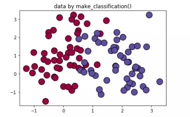
plt.title('data by make_classification()')
plt.show()
数据分布展示如下:
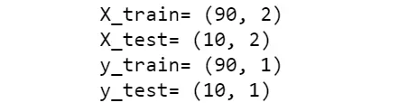
对数据进行简单的训练集与测试集的划分:
offset = int(X.shape[0] * 0.9)
X_train, y_train = X[:offset], labels[:offset]
X_test, y_test = X[offset:], labels[offset:]
y_train = y_train.reshape((-1,1))
y_test = y_test.reshape((-1,1))

print('X_train=', X_train.shape)
print('X_test=', X_test.shape)
print('y_train=', y_train.shape)
print('y_test=', y_test.shape)
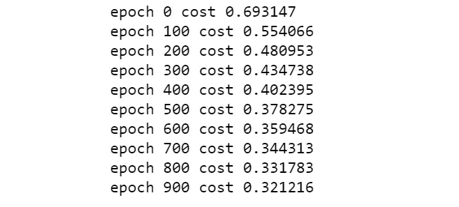
对训练集进行训练:
cost_list, params, grads = lr_train(X_train, y_train, 0.01, 1000)
迭代过程如下:
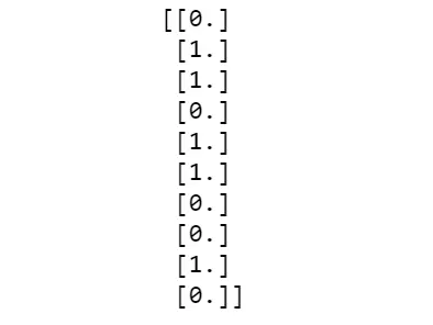
对测试集数据进行预测:
y_prediction = predict(X_test, params)
print(y_prediction)
预测结果如下:
定义一个分类准确率函数对训练集和测试集的准确率进行评估:
def accuracy(y_test, y_pred):
correct_count = 0
for i in range(len(y_test)):
for j in range(len(y_pred)):
if y_test[i] == y_pred[j] and i == j:
correct_count +=1
accuracy_score = correct_count / len(y_test)
return accuracy_score
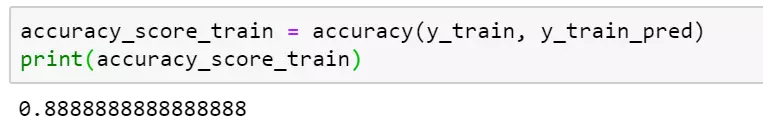
# 打印训练准确率
accuracy_score_train = accuracy(y_train, y_train_pred)
print(accuracy_score_train)
查看测试集准确率:
accuracy_score_test = accuracy(y_test, y_prediction)
print(accuracy_score_test)
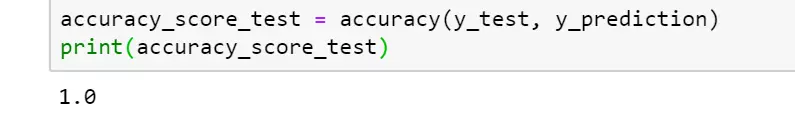
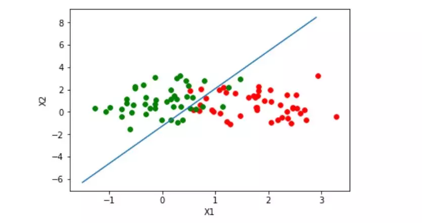
没有进行交叉验证,测试集准确率存在一定的偶然性哈。 最后我们定义个绘制模型决策边界的图形函数对训练结果进行可视化展示:
def plot_logistic(X_train, y_train, params):
    n = X_train.shape[0]
    xcord1 = []
    ycord1 = []
    xcord2 = []
    ycord2 = []
    for i in range(n):
        if y_train[i] == 1:
            xcord1.append(X_train[i][0])
            ycord1.append(X_train[i][1])
        else:
            xcord2.append(X_train[i][0])
            ycord2.append(X_train[i][1])

    fig = plt.figure()
    ax = fig.add_subplot(111)
    ax.scatter(xcord1, ycord1,s=32, c='red')
    ax.scatter(xcord2, ycord2, s=32, c='green')
    x = np.arange(-1.5, 3, 0.1)
    y = (-params['b'] - params['W'][0] * x) / params['W'][1]
    ax.plot(x, y)
    plt.xlabel('X1')
    plt.ylabel('X2')
    plt.show()

plot_logistic(X_train, y_train, params)
组件封装成逻辑回归类
将以上实现过程使用一个 python 类进行封装:
import numpy as np
import matplotlib.pyplot as plt
from sklearn.datasets.samples_generator import make_classification

class logistic_regression():
    def __init__(self):
        pass

    def sigmoid(self, x):
        z = 1 / (1 + np.exp(-x))
        return z

    def initialize_params(self, dims):
        W = np.zeros((dims, 1))
        b = 0
        return W, b

    def logistic(self, X, y, W, b):
        num_train = X.shape[0]
        num_feature = X.shape[1]

        a = self.sigmoid(np.dot(X, W) + b)
        cost = -1 / num_train * np.sum(y * np.log(a) + (1 - y) * np.log(1 - a))

        dW = np.dot(X.T, (a - y)) / num_train
        db = np.sum(a - y) / num_train
        cost = np.squeeze(cost)
        return a, cost, dW, db

    def logistic_train(self, X, y, learning_rate, epochs):
        W, b = self.initialize_params(X.shape[1])
        cost_list = []
        for i in range(epochs):
            a, cost, dW, db = self.logistic(X, y, W, b)
            W = W - learning_rate * dW
            b = b - learning_rate * db
            if i % 100 == 0:
                cost_list.append(cost)
            if i % 100 == 0:
                print('epoch %d cost %f' % (i, cost))

        params = {
            'W': W,
            'b': b
        }
        grads = {
            'dW': dW,
            'db': db
        }

        return cost_list, params, grads

    def predict(self, X, params):
        y_prediction = self.sigmoid(np.dot(X, params['W']) + params['b'])
        for i in range(len(y_prediction)):
            if y_prediction[i] > 0.5:
                y_prediction[i] = 1
            else:
                y_prediction[i] = 0

        return y_prediction

    def accuracy(self, y_test, y_pred):
        correct_count = 0
        for i in range(len(y_test)):
            for j in range(len(y_pred)):
                if y_test[i] == y_pred[j] and i == j:
                    correct_count += 1

        accuracy_score = correct_count / len(y_test)
        return accuracy_score

    def create_data(self):
        X, labels = make_classification(n_samples=100, n_features=2, n_redundant=0, n_informative=2, random_state=1, n_clusters_per_class=2)
        labels = labels.reshape((-1, 1))
        offset = int(X.shape[0] * 0.9)
        X_train, y_train = X[:offset], labels[:offset]
        X_test, y_test = X[offset:], labels[offset:]
        return X_train, y_train, X_test, y_test

    def plot_logistic(self, X_train, y_train, params):
        n = X_train.shape[0]
        xcord1 = []
        ycord1 = []
        xcord2 = []
        ycord2 = []
        for i in range(n):
            if y_train[i] == 1:
                xcord1.append(X_train[i][0])
                ycord1.append(X_train[i][1])
            else:
                xcord2.append(X_train[i][0])
                ycord2.append(X_train[i][1])
        fig = plt.figure()
        ax = fig.add_subplot(111)
        ax.scatter(xcord1, ycord1, s=32, c='red')
        ax.scatter(xcord2, ycord2, s=32, c='green')
        x = np.arange(-1.5, 3, 0.1)
        y = (-params['b'] - params['W'][0] * x) / params['W'][1]
        ax.plot(x, y)
        plt.xlabel('X1')
        plt.ylabel('X2')
       plt.show()


if __name__ == "__main__":
    model = logistic_regression()
    X_train, y_train, X_test, y_test = model.create_data()
    print(X_train.shape, y_train.shape, X_test.shape, y_test.shape)
    cost_list, params, grads = model.logistic_train(X_train, y_train, 0.01, 1000)
    print(params)
    y_train_pred = model.predict(X_train, params)
    accuracy_score_train = model.accuracy(y_train, y_train_pred)
    print('train accuracy is:', accuracy_score_train)
    y_test_pred = model.predict(X_test, params)
    accuracy_score_test = model.accuracy(y_test, y_test_pred)
    print('test accuracy is:', accuracy_score_test)
    model.plot_logistic(X_train, y_train, params)
好了,关于逻辑回归的内容,笔者就介绍到这,至于如何在实战中检验逻辑回归的分类效果,还需各位亲自试一试。多说一句,逻辑回归模型与感知机、神经网络和深度学习有着千丝万缕的关系,作为基础的机器学习模型,希望大家能够牢固掌握其数学推导和手动实现方式,在此基础上再去调用 sklearn 中的 LogisticRegression 模块,必能必能裨补阙漏,有所广益。
参考资料:
