

10.13 Update:最近新出了一个state-of-the-art预训练模型,传送门:
李入魔:【NLP】Google BERT详解zhuanlan.zhihu.com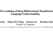
1. 简介
长期以来,词向量一直是NLP任务中的主要表征技术。随着2017年底以及2018年初的一系列技术突破,研究证实预训练的语言表征经过精调后可以在众多NLP任务中达到更好的表现。目前预训练有两种方法:
- Feature-based:将训练出的representation作为feature用于任务,从词向量、句向量、段向量、文本向量都是这样的。新的ELMo也属于这类,但迁移后需要重新计算出输入的表征。
- Fine-tuning:这个主要借鉴于CV,就是在预训练好的模型上加些针对任务的层,再对后几层进行精调。新的ULMFit和OpenAI GPT属于这一类。
本文主要对ELMo、ULMFiT以及OpenAI GPT三种预训练语言模型作简要介绍。
2. ELMo
2.1 模型原理与架构
原文链接:Deep contextualized word representations
ELMo是从双向语言模型(BiLM)中提取出的Embedding。训练时使用BiLSTM,给定N个tokens (t1, t2,...,tN), 目标为最大化:

ELMo对于每个token  , 通过一个L层的biLM计算出2L+1个表示:

其中  是对token进行直接编码的结果(这里是字符通过CNN编码),
 ![h_{k,j}^{LM} = [\overrightarrow{h}{k,j}^{LM}; \overleftarrow{h}{k, j}^{LM}]](https://p1-jj.byteimg.com/tos-cn-i-t2oaga2asx/gold-user-assets/2018/11/30/16762948ec6c79f7~tplv-t2oaga2asx-jj-mark:3024:0:0:0:q75.png) 是每个biLSTM层输出的结果。
是每个biLSTM层输出的结果。
应用中将ELMo中所有层的输出R压缩为单个向量,  , 最简单的压缩方法是取最上层的结果做为token的表示:
  , 更通用的做法是通过一些参数来联合所有层的信息:

其中  是softmax出来的权重,
 是一个任务相关的scale参数,在优化过程中很重要,同时因为每层BiLM的输出分布不同,
  可以对层起到normalisation的作用。
论文中使用的预训练BiLM在Jozefowicz et al.中的CNN-BIG-LSTM基础上做了修改,最终模型为2层biLSTM(4096 units, 512 dimension projections),并在第一层和第二层之间增加了残差连接。同时使用CNN和两层Highway对token进行字符级的上下文无关编码。使得模型最终对每个token输出三层向量表示。
2.2 模型训练注意事项
- 正则化:
1. Dropout
2. 在loss中添加权重的惩罚项  (实验结果显示ELMo适合较小的
  )
)
- TF版源码解析:
1. 模型架构的代码主要在training模块的LanguageModel类中,分为两步:第一步创建word或character的Embedding层(CNN+Highway);第二步创建BiLSTM层。
2. 加载所需的预训练模型为model模块中的BidirectionalLanguageModel类。
2.3 模型的使用
- 将ELMo向量
 与传统的词向量
  拼接成
拼接成 ![[x_{k};ELMo_k^{task}]](https://p1-jj.byteimg.com/tos-cn-i-t2oaga2asx/gold-user-assets/2018/11/30/167629491087c238~tplv-t2oaga2asx-jj-mark:3024:0:0:0:q75.png) 后,输入到对应具体任务的RNN中。
后,输入到对应具体任务的RNN中。 - 将ELMo向量放到模型输出部分,与具体任务RNN输出的
 拼接成
拼接成 ![[h_{k};ELMo_k^{task}]](https://p1-jj.byteimg.com/tos-cn-i-t2oaga2asx/gold-user-assets/2018/11/30/16762948feef18c0~tplv-t2oaga2asx-jj-mark:3024:0:0:0:q75.png) 。
。 - Keras代码示例
import tensorflow as tf
from keras import backend as K
import keras.layers as layers
from keras.models import Model

# Initialize session
sess = tf.Session()
K.set_session(sess)

# Instantiate the elmo model
elmo_model = hub.Module("https://tfhub.dev/google/elmo/1", trainable=True)
sess.run(tf.global_variables_initializer())
sess.run(tf.tables_initializer())

# We create a function to integrate the tensorflow model with a Keras model
# This requires explicitly casting the tensor to a string, because of a Keras quirk
def ElmoEmbedding(x):
    return elmo_model(tf.squeeze(tf.cast(x, tf.string)), signature="default", as_dict=True)["default"]

input_text = layers.Input(shape=(1,), dtype=tf.string)
embedding = layers.Lambda(ElmoEmbedding, output_shape=(1024,))(input_text)
dense = layers.Dense(256, activation='relu')(embedding)
pred = layers.Dense(1, activation='sigmoid')(dense)

model = Model(inputs=[input_text], outputs=pred)

model.compile(loss='binary_crossentropy', optimizer='adam', metrics=['accuracy'])
model.summary()
2.4 模型的优缺点
优点:
- 效果好,在大部分任务上都较传统模型有提升。实验正式ELMo相比于词向量,可以更好地捕捉到语法和语义层面的信息。
- 传统的预训练词向量只能提供一层表征,而且词汇量受到限制。ELMo所提供的是character-level的表征,对词汇量没有限制。
缺点:
速度较慢,对每个token编码都要通过language model计算得出。
2.5 适用任务
- Question Answering
- Textual entailment
- Semantic role labeling
- Coreference resolution
- Named entity extraction
- Sentiment analysis
3. ULMFiT
3.1 模型原理与架构
原文链接:Universal Language Model Fine-tuning for Text Classification
ULMFiT是一种有效的NLP迁移学习方法,核心思想是通过精调预训练的语言模型完成其他NLP任务。文中所用的语言模型参考了Merity et al. 2017a的AWD-LSTM模型,即没有attention或shortcut的三层LSTM模型。
ULMFiT的过程分为三步:
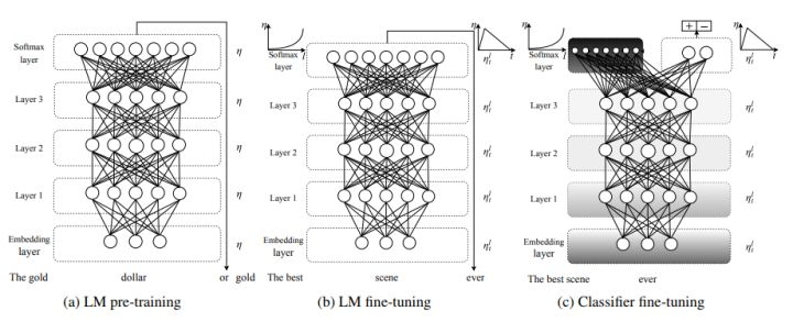
1. General-domain LM pre-train
- 在Wikitext-103上进行语言模型的预训练。
- 预训练的语料要求:large & capture general properties of language
- 预训练对小数据集十分有效,之后仅有少量样本就可以使模型泛化。
2. Target task LM fine-tuning
文中介绍了两种fine-tuning方法:
- Discriminative fine-tuning
因为网络中不同层可以捕获不同类型的信息,因此在精调时也应该使用不同的learning rate。作者为每一层赋予一个学习率  ,实验后发现,首先通过精调模型的最后一层L确定学习率
  ,再递推地选择上一层学习率进行精调的效果最好,递推公式为:
- Slanted triangular learning rates (STLR)
为了针对特定任务选择参数,理想情况下需要在训练开始时让参数快速收敛到一个合适的区域,之后进行精调。为了达到这种效果,作者提出STLR方法,即让LR在训练初期短暂递增,在之后下降。如图b的右上角所示。具体的公式为:


- T: number of training iterations
- cut_frac: fraction of iterations we increase the LR
- cut: the iteration when we switch from increasing to decreasing the LR
- p: the fraction of the number of iterations we have increased or will decrease the LR respectively
- ratio: specifies how much smaller the lowest LR is from thr max LR

 : the LR at iteration t
文中作者使用的 
3. Target task classifier fine-tuning
为了完成分类任务的精调,作者在最后一层添加了两个线性block,每个都有batch-norm和dropout,使用ReLU作为中间层激活函数,最后经过softmax输出分类的概率分布。最后的精调涉及的环节如下:
- Concat pooling
第一个线性层的输入是最后一个隐层状态的池化。因为文本分类的关键信息可能在文本的任何地方,所以只是用最后时间步的输出是不够的。作者将最后时间步 与尽可能多的时间步
  池化后拼接起来,以
 ![h_{c} = [h_{T}, maxpool(H), meanpool(H)]](https://p1-jj.byteimg.com/tos-cn-i-t2oaga2asx/gold-user-assets/2018/11/30/1676294900544401~tplv-t2oaga2asx-jj-mark:3024:0:0:0:q75.png) 作为输入。
作为输入。
- Gradual unfreezing
由于过度精调会导致模型遗忘之前预训练得到的信息,作者提出逐渐unfreez网络层的方法,从最后一层开始unfreez和精调,由后向前地unfreez并精调所有层。
- BPTT for Text Classification (BPT3C)
为了在large documents上进行模型精调,作者将文档分为固定长度为b的batches,并在每个batch训练时记录mean和max池化,梯度会被反向传播到对最终预测有贡献的batches。
- Bidirectional language model
在作者的实验中,分别独立地对前向和后向LM做了精调,并将两者的预测结果平均。两者结合后结果有0.5-0.7的提升。
3.2 模型训练注意事项
- PyTorch版源码解析 (FastAI第10课)
# location: fastai/lm_rnn.py

def get_language_model(n_tok, emb_sz, n_hid, n_layers, pad_token,
                 dropout=0.4, dropouth=0.3, dropouti=0.5, dropoute=0.1, wdrop=0.5, tie_weights=True, qrnn=False, bias=False):
    """Returns a SequentialRNN model.

    A RNN_Encoder layer is instantiated using the parameters provided.

    This is followed by the creation of a LinearDecoder layer.

    Also by default (i.e. tie_weights = True), the embedding matrix used in the RNN_Encoder
    is used to  instantiate the weights for the LinearDecoder layer.

    The SequentialRNN layer is the native torch's Sequential wrapper that puts the RNN_Encoder and
    LinearDecoder layers sequentially in the model.

    Args:
        n_tok (int): number of unique vocabulary words (or tokens) in the source dataset
        emb_sz (int): the embedding size to use to encode each token
        n_hid (int): number of hidden activation per LSTM layer
        n_layers (int): number of LSTM layers to use in the architecture
        pad_token (int): the int value used for padding text.
        dropouth (float): dropout to apply to the activations going from one LSTM layer to another
        dropouti (float): dropout to apply to the input layer.
        dropoute (float): dropout to apply to the embedding layer.
        wdrop (float): dropout used for a LSTM's internal (or hidden) recurrent weights.
        tie_weights (bool): decide if the weights of the embedding matrix in the RNN encoder should be tied to the
            weights of the LinearDecoder layer.
        qrnn (bool): decide if the model is composed of LSTMS (False) or QRNNs (True).
        bias (bool): decide if the decoder should have a bias layer or not.
    Returns:
        A SequentialRNN model
    """
    rnn_enc = RNN_Encoder(n_tok, emb_sz, n_hid=n_hid, n_layers=n_layers, pad_token=pad_token,
                 dropouth=dropouth, dropouti=dropouti, dropoute=dropoute, wdrop=wdrop, qrnn=qrnn)
    enc = rnn_enc.encoder if tie_weights else None
    return SequentialRNN(rnn_enc, LinearDecoder(n_tok, emb_sz, dropout, tie_encoder=enc, bias=bias))


def get_rnn_classifier(bptt, max_seq, n_class, n_tok, emb_sz, n_hid, n_layers, pad_token, layers, drops, bidir=False,
                      dropouth=0.3, dropouti=0.5, dropoute=0.1, wdrop=0.5, qrnn=False):
    rnn_enc = MultiBatchRNN(bptt, max_seq, n_tok, emb_sz, n_hid, n_layers, pad_token=pad_token, bidir=bidir,
                      dropouth=dropouth, dropouti=dropouti, dropoute=dropoute, wdrop=wdrop, qrnn=qrnn)
    return SequentialRNN(rnn_enc, PoolingLinearClassifier(layers, drops))
3.3 模型的优缺点
优点:
对比其他迁移学习方法(ELMo)更适合以下任务:
- 非英语语言,有标签训练数据很少
- 没有state-of-the-art模型的新NLP任务
- 只有部分有标签数据的任务
缺点:
对于分类和序列标注任务比较容易迁移,对于复杂任务(问答等)需要新的精调方法。
3.4 适用任务
- Classification
- Sequence labeling
4. OpenAI GPT
4.1 模型原理与架构
原文链接:Improving Language Understanding by Generative Pre-Training (未出版)
OpenAI Transformer是一类可迁移到多种NLP任务的,基于Transformer的语言模型。它的基本思想同ULMFiT相同,都是在尽量不改变模型结构的情况下将预训练的语言模型应用到各种任务。不同的是,OpenAI Transformer主张用Transformer结构,而ULMFiT中使用的是基于RNN的语言模型。文中所用的网络结构如下:
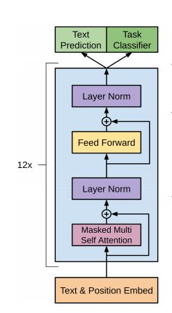
模型的训练过程分为两步:
1. Unsupervised pre-training
第一阶段的目标是预训练语言模型,给定tokens的语料  ,目标函数为最大化似然函数:

该模型中应用multi-headed self-attention,并在之后增加position-wise的前向传播层,最后输出一个分布:


2. Supervised fine-tuning
有了预训练的语言模型之后,对于有标签的训练集  ,给定输入序列
  和标签
和标签  ,可以通过语言模型得到
  ,经过输出层后对
  进行预测:
进行预测:

则目标函数为:

整个任务的目标函数为:

4.2 模型训练注意事项
- TF版源码解析
# location: finetune-transformer-lm/train.py

def model(X, M, Y, train=False, reuse=False):
    with tf.variable_scope('model', reuse=reuse):
        # n_special=3,作者把数据集分为三份
        # n_ctx 应该是 n_context
        we = tf.get_variable("we", [n_vocab+n_special+n_ctx, n_embd], initializer=tf.random_normal_initializer(stddev=0.02))
        we = dropout(we, embd_pdrop, train)

        X = tf.reshape(X, [-1, n_ctx, 2])
        M = tf.reshape(M, [-1, n_ctx])

        # 1. Embedding
        h = embed(X, we)

        # 2. transformer block
        for layer in range(n_layer):
            h = block(h, 'h%d'%layer, train=train, scale=True)

        # 3. 计算语言模型loss
        lm_h = tf.reshape(h[:, :-1], [-1, n_embd])
        lm_logits = tf.matmul(lm_h, we, transpose_b=True)
        lm_losses = tf.nn.sparse_softmax_cross_entropy_with_logits(logits=lm_logits, labels=tf.reshape(X[:, 1:, 0], [-1]))
        lm_losses = tf.reshape(lm_losses, [shape_list(X)[0], shape_list(X)[1]-1])
        lm_losses = tf.reduce_sum(lm_losses*M[:, 1:], 1)/tf.reduce_sum(M[:, 1:], 1)

        # 4. 计算classifier loss
        clf_h = tf.reshape(h, [-1, n_embd])
        pool_idx = tf.cast(tf.argmax(tf.cast(tf.equal(X[:, :, 0], clf_token), tf.float32), 1), tf.int32)
        clf_h = tf.gather(clf_h, tf.range(shape_list(X)[0], dtype=tf.int32)*n_ctx+pool_idx)

        clf_h = tf.reshape(clf_h, [-1, 2, n_embd])
        if train and clf_pdrop > 0:
            shape = shape_list(clf_h)
            shape[1] = 1
            clf_h = tf.nn.dropout(clf_h, 1-clf_pdrop, shape)
        clf_h = tf.reshape(clf_h, [-1, n_embd])
        clf_logits = clf(clf_h, 1, train=train)
        clf_logits = tf.reshape(clf_logits, [-1, 2])

        clf_losses = tf.nn.sparse_softmax_cross_entropy_with_logits(logits=clf_logits, labels=Y)
        return clf_logits, clf_losses, lm_losses
4.3 模型的优缺点
优点:
- 循环神经网络所捕捉到的信息较少,而Transformer可以捕捉到更长范围的信息。
- 计算速度比循环神经网络更快,易于并行化
- 实验结果显示Transformer的效果比ELMo和LSTM网络更好
缺点:
对于某些类型的任务需要对输入数据的结构作调整
4.4 适用任务
- Natural Language Inference
- Question Answering and commonsense reasoning
- Classification
- Semantic Similarity
5. 总结
从Wrod Embedding到OpenAI Transformer,NLP中的迁移学习从最初使用word2vec、GLoVe进行字词的向量表示,到ELMo可以提供前几层的权重共享,再到ULMFiT和OpenAI Transformer的整个预训练模型的精调,大大提高了NLP基本任务的效果。同时,多项研究也表明,以语言模型作为预训练模型,不仅可以捕捉到文字间的语法信息,更可以捕捉到语义信息,为后续的网络层提供高层次的抽象信息。另外,基于Transformer的模型在一些方面也展现出了优于RNN模型的效果。
最后,关于具体任务还是要进行多种尝试,可以使用以上方法做出模型baseline,再调整网络结构提升效果。
