

1、什么是 RDD?
上一章讲了 Spark 提交作业的过程,这一章我们要讲 RDD。简单的讲,RDD 就是 Spark 的 input,知道 input 是啥吧,就是输入的数据。
RDD 的全名是 Resilient Distributed Dataset,意思是容错的分布式数据集,每一个 RDD 都会有 5 个特征:
1、有一个分片列表。就是能被切分,和 hadoop 一样的,能够切分的数据才能并行计算。
2、有一个函数计算每一个分片,这里指的是下面会提到的 compute 函数。
3、对其他的 RDD 的依赖列表,依赖还具体分为宽依赖和窄依赖,但并不是所有的 RDD 都有依赖。
4、可选:key-value 型的 RDD 是根据哈希来分区的,类似于 mapreduce 当中的 Paritioner 接口,控制 key 分到哪个 reduce。
5、可选:每一个分片的优先计算位置(preferred locations),比如 HDFS 的 block 的所在位置应该是优先计算的位置。
对应着上面这几点,我们在 RDD 里面能找到这 4 个方法和 1 个属性,别着急,下面我们会慢慢展开说这 5 个东东。
  //只计算一次
  protected def getPartitions: Array[Partition]
  //对一个分片进行计算,得出一个可遍历的结果
  def compute(split: Partition, context: TaskContext): Iterator[T]
  //只计算一次,计算RDD对父RDD的依赖
  protected def getDependencies: Seq[Dependency[_]] = deps
  //可选的,分区的方法,针对第4点,类似于mapreduce当中的Paritioner接口,控制key分到哪个reduce
  @transient val partitioner: Option[Partitioner] = None
  //可选的,指定优先位置,输入参数是split分片,输出结果是一组优先的节点位置
  protected def getPreferredLocations(split: Partition): Seq[String] = Nil
2、多种 RDD 之间的转换
下面用一个实例讲解一下吧,就拿我们常用的一段代码来讲吧,然后会把我们常用的 RDD 都会讲到。
    val hdfsFile = sc.textFile(args(1))
    val flatMapRdd = hdfsFile.flatMap(s => s.split(" "))
    val filterRdd = flatMapRdd.filter(_.length == 2)
    val mapRdd = filterRdd.map(word => (word, 1))
    val reduce = mapRdd.reduceByKey(_ + _)
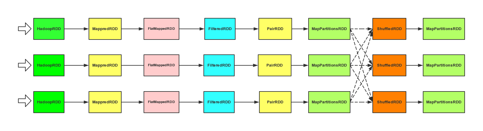
这里涉及到很多个 RDD,textFile 是一个 HadoopRDD 经过 map 后的 MappredRDD,经过 flatMap 是一个 FlatMappedRDD,经过 filter 方法之后生成了一个 FilteredRDD,经过 map 函数之后,变成一个 MappedRDD,通过隐式转换成 PairRDD,最后经过 reduceByKey。
我们首先看 textFile 的这个方法,进入 SparkContext 这个方法,找到它。
def textFile(path: String, minPartitions: Int = defaultMinPartitions): RDD[String] = {
    hadoopFile(path, classOf[TextInputFormat], classOf[LongWritable], classOf[Text], minPartitions).map(pair => pair._2.toString)
}
看它的输入参数,path,TextInputFormat,LongWritable,Text,同志们联想到什么?写过 mapreduce 的童鞋都应该知道哈。
1、hdfs 的地址
2、InputFormat 的类型
3、Mapper 的第一个类型
4、Mapper 的第二类型
这就不难理解为什么立马就对 hadoopFile 后面加了一个 map 方法,取 pair 的第二个参数了,最后在 shell 里面我们看到它是一个 MappredRDD 了。
那么现在如果大家要用的不是 textFile,而是一个别的 hadoop 文件类型,大家会不会使用 hadoopFile 来得到自己要得到的类型呢,不要告诉我不会哈,不会的赶紧回去复习 mapreduce。
言归正传,默认的 defaultMinPartitions 的 2 太小了,我们用的时候还是设置大一点吧。
2.1 HadoopRDD
我们继续追杀下去,看看 hadoopFile 方法,里面我们看到它做了 3 个操作。
1、把 hadoop 的配置文件保存到广播变量里。
2、设置路径的方法
3、new 了一个 HadoopRDD 返回
好,我们接下去看看 HadoopRDD 这个类吧,我们重点看看它的 getPartitions、compute、getPreferredLocations。
先看 getPartitions,它的核心代码如下:
    val inputSplits = inputFormat.getSplits(jobConf, minPartitions)
    val array = new Array[Partition](inputSplits.size)
    for (i <- 0 until inputSplits.size) {
      array(i) = new HadoopPartition(id, i, inputSplits(i))
    }
它调用的是 inputFormat 自带的 getSplits 方法来计算分片,然后把分片 HadoopPartition 包装到到 array 里面返回。
这里顺便顺带提一下,因为 1.0 又出来一个 NewHadoopRDD,它使用的是 mapreduce 新 api 的 inputformat,getSplits 就不要有 minPartitions 了,别的逻辑都是一样的,只是使用的类有点区别。
我们接下来看 compute 方法,它的输入值是一个 Partition,返回是一个 Iterator[(K, V)] 类型的数据,这里面我们只需要关注 2 点即可。
1、把 Partition 转成 HadoopPartition,然后通过 InputSplit 创建一个 RecordReader
2、重写 Iterator 的 getNext 方法,通过创建的 reader 调用 next 方法读取下一个值。
      // 转换成HadoopPartition
      val split = theSplit.asInstanceOf[HadoopPartition]
      logInfo("Input split: " + split.inputSplit)
      var reader: RecordReader[K, V] = null
      val jobConf = getJobConf()
      val inputFormat = getInputFormat(jobConf)
        context.stageId, theSplit.index, context.attemptId.toInt, jobConf)
      // 通过Inputform的getRecordReader来创建这个InputSpit的Reader
      reader = inputFormat.getRecordReader(split.inputSplit.value, jobConf, Reporter.NULL)

      // 调用Reader的next方法
      val key: K = reader.createKey()
      val value: V = reader.createValue()
      override def getNext() = {
        try {
          finished = !reader.next(key, value)
        } catch {
          case eof: EOFException =>
            finished = true
        }
        (key, value)
      }
从这里我们可以看得出来 compute 方法是通过分片来获得 Iterator 接口,以遍历分片的数据。
getPreferredLocations 方法就更简单了,直接调用 InputSplit 的 getLocations 方法获得所在的位置。
2.2 依赖
下面我们看 RDD 里面的 map 方法
def map[U: ClassTag](f: T => U): RDD[U] = new MappedRDD(this, sc.clean(f))
直接 new 了一个 MappedRDD,还把匿名函数 f 处理了再传进去,我们继续追杀到 MappedRDD。
private[spark]
class MappedRDD[U: ClassTag, T: ClassTag](prev: RDD[T], f: T => U)
  extends RDD[U](prev) {
  override def getPartitions: Array[Partition] = firstParent[T].partitions
  override def compute(split: Partition, context: TaskContext) =
    firstParent[T].iterator(split, context).map(f)
}
MappedRDD 把 getPartitions 和 compute 给重写了,而且都用到了 firstParent[T],这个 firstParent 是何须人也?我们可以先点击进入 RDDU 这个构造函数里面去。
def this(@transient oneParent: RDD[_]) = this(oneParent.context , List(new OneToOneDependency(oneParent)))
就这样你会发现它把 RDD 复制给了 deps,HadoopRDD 成了 MappedRDD 的父依赖了,这个 OneToOneDependency 是一个窄依赖,子 RDD 直接依赖于父 RDD,继续看 firstParent。
protected[spark] def firstParent[U: ClassTag] = {
  dependencies.head.rdd.asInstanceOf[RDD[U]]
}
由此我们可以得出两个结论:
1、getPartitions 直接沿用了父 RDD 的分片信息
2、compute 函数是在父 RDD 遍历每一行数据时套一个匿名函数 f 进行处理
好吧,现在我们可以理解 compute 函数真正是在干嘛的了
它的两个显著作用:
1、在没有依赖的条件下,根据分片的信息生成遍历数据的 Iterable 接口
2、在有前置依赖的条件下,在父 RDD 的 Iterable 接口上给遍历每个元素的时候再套上一个方法
我们看看点击进入 map(f) 的方法进去看一下
  def map[B](f: A => B): Iterator[B] = new AbstractIterator[B] {
    def hasNext = self.hasNext
    def next() = f(self.next())
  }
看黄色的位置,看它的 next 函数,不得不说,写得真的很妙!
我们接着看 RDD 的 flatMap 方法,你会发现它和 map 函数几乎没什么区别,只是 RDD 变成了 FlatMappedRDD,但是 flatMap 和 map 的效果还是差别挺大的。
比如 ((1,2),(3,4)), 如果是调用了 flatMap 函数,我们访问到的就是(1,2,3,4)4 个元素;如果是 map 的话,我们访问到的就是(1,2),(3,4) 两个元素。
有兴趣的可以去看看 FlatMappedRDD 和 FilteredRDD 这里就不讲了,和 MappedRDD 类似。
2.3 reduceByKey
前面的 RDD 转换都简单,可是到了 reduceByKey 可就不简单了哦,因为这里有一个同相同 key 的内容聚合的一个过程,所以它是最复杂的那一类。
那 reduceByKey 这个方法在哪里呢,它在 PairRDDFunctions 里面,这是个隐式转换,所以比较隐蔽哦,你在 RDD 里面是找不到的。
  def reduceByKey(partitioner: Partitioner, func: (V, V) => V): RDD[(K, V)] = {
    combineByKey[V]((v: V) => v, func, func, partitioner)
  }
它调用的是 combineByKey 方法,过程过程蛮复杂的,折叠起来,喜欢看的人看看吧。
def combineByKey[C](createCombiner: V => C,
      mergeValue: (C, V) => C,
      mergeCombiners: (C, C) => C,
      partitioner: Partitioner,
      mapSideCombine: Boolean = true,
      serializer: Serializer = null): RDD[(K, C)] = {

    val aggregator = new Aggregator[K, V, C](createCombiner, mergeValue, mergeCombiners)
    if (self.partitioner == Some(partitioner)) {
      // 一般的RDD的partitioner是None,这个条件不成立,即使成立只需要对这个数据做一次按key合并value的操作即可
      self.mapPartitionsWithContext((context, iter) => {
        new InterruptibleIterator(context, aggregator.combineValuesByKey(iter, context))
      }, preservesPartitioning = true)
    } else if (mapSideCombine) {
      // 默认是走的这个方法,需要map端的combinber.
      val combined = self.mapPartitionsWithContext((context, iter) => {
        aggregator.combineValuesByKey(iter, context)
      }, preservesPartitioning = true)
      val partitioned = new ShuffledRDD[K, C, (K, C)](combined, partitioner)
        .setSerializer(serializer)
      partitioned.mapPartitionsWithContext((context, iter) => {
        new InterruptibleIterator(context, aggregator.combineCombinersByKey(iter, context))
      }, preservesPartitioning = true)
    } else {
      // 不需要map端的combine,直接就来shuffle
      val values = new ShuffledRDD[K, V, (K, V)](self, partitioner).setSerializer(serializer)
      values.mapPartitionsWithContext((context, iter) => {
        new InterruptibleIterator(context, aggregator.combineValuesByKey(iter, context))
      }, preservesPartitioning = true)
    }
  }
按照一个比较标准的流程来看的话,应该是走的中间的这条路径,它干了三件事:
1、给每个分片的数据在外面套一个 combineValuesByKey 方法的 MapPartitionsRDD。
2、用 MapPartitionsRDD 来 new 了一个 ShuffledRDD 出来。
3、对 ShuffledRDD 做一次 combineCombinersByKey。
下面我们先看 MapPartitionsRDD,我把和别的 RDD 有别的两行给拿出来了,很明显的区别,f 方法是套在 iterator 的外边,这样才能对 iterator 的所有数据做一个合并。
  override val partitioner = if (preservesPartitioning) firstParent[T].partitioner else None
  override def compute(split: Partition, context: TaskContext) =
    f(context, split.index, firstParent[T].iterator(split, context))
}
接下来我们看 Aggregator 的 combineValuesByKey 的方法吧。
def combineValuesByKey(iter: Iterator[_ <: Product2[K, V]],
                         context: TaskContext): Iterator[(K, C)] = {
    // 是否使用外部排序,是由参数spark.shuffle.spill,默认是true
    if (!externalSorting) {
      val combiners = new AppendOnlyMap[K,C]
      var kv: Product2[K, V] = null
      val update = (hadValue: Boolean, oldValue: C) => {
        if (hadValue) mergeValue(oldValue, kv._2) else createCombiner(kv._2)
      }
      // 用map来去重,用update方法来更新值,如果没值的时候,返回值,如果有值的时候,通过mergeValue方法来合并
      // mergeValue方法就是我们在reduceByKey里面写的那个匿名函数,在这里就是(_ + _)
      while (iter.hasNext) {
        kv = iter.next()
        combiners.changeValue(kv._1, update)
      }
      combiners.iterator
    } else {
      // 用了一个外部排序的map来去重,就不停的往里面插入值即可,基本原理和上面的差不多,区别在于需要外部排序
      val combiners = new ExternalAppendOnlyMap[K, V, C](createCombiner, mergeValue, mergeCombiners)
      while (iter.hasNext) {
        val (k, v) = iter.next()
        combiners.insert(k, v)
      }
      combiners.iterator
}
View Code
这个就是一个很典型的按照 key 来做合并的方法了,我们继续看 ShuffledRDD 吧。
ShuffledRDD 和之前的 RDD 很明显的特征是
1、它的依赖传了一个 Nil(空列表)进去,表示它没有依赖。
2、它的 compute 计算方式比较特别,这个在之后的文章说,过程比较复杂。
3、它的分片默认是采用 HashPartitioner,数量和前面的 RDD 的分片数量一样,也可以不一样,我们可以在 reduceByKey 的时候多传一个分片数量即可。
在 new 完 ShuffledRDD 之后又来了一遍 mapPartitionsWithContext,不过调用的匿名函数变成了 combineCombinersByKey。
combineCombinersByKey 和 combineValuesByKey 的逻辑基本相同,只是输入输出的类型有区别。combineCombinersByKey 只是做单纯的合并,不会对输入输出的类型进行改变,combineValuesByKey 会把 iter[K, V] 的 V 值变成 iter[K, C]。
case class Aggregator[K, V, C] (
  createCombiner: V => C,
  mergeValue: (C, V) => C,
  mergeCombiners: (C, C) => C)
  ......
}
这个方法会根据我们传进去的匿名方法的参数的类型做一个自动转换。
到这里,作业都没有真正执行,只是将 RDD 各种嵌套,我们通过 RDD 的 id 和类型的变化观测到这一点,RDD[1]->RDD[2]->RDD[3]......
3、其它RDD
平常我们除了从 hdfs 上面取数据之后,我们还可能从数据库里面取数据,那怎么办呢?没关系,有个 JdbcRDD!
    val rdd = new JdbcRDD(
      sc,
      () => { DriverManager.getConnection("jdbc:derby:target/JdbcRDDSuiteDb") },
      "SELECT DATA FROM FOO WHERE ? <= ID AND ID <= ?",
      1, 100, 3,
      (r: ResultSet) => { r.getInt(1) }
   ).cache()
前几个参数大家都懂,我们重点说一下后面 1, 100, 3 是咋回事?
在这个 JdbcRDD 里面它默认我们是会按照一个 long 类型的字段对数据进行切分,(1,100)分别是最小值和最大值,3 是分片的数量。
比如我们要一次查 ID 为 1-1000,000 的的用户,分成 10 个分片,我们就填(1, 1000,000, 10)即可,在 sql 语句里面还必须有 "? <= ID AND ID <= ?" 的句式,别尝试着自己造句哦!
最后是怎么处理 ResultSet 的方法,自己爱怎么处理怎么处理去吧。不过确实觉着用得不方便的可以自己重写一个 RDD。
小结:
这一章重点介绍了各种 RDD 那 5 个特征,以及 RDD 之间的转换,希望大家可以对 RDD 有更深入的了解,下一章我们将要讲作业的运行过程,敬请关注!
