1. 介绍
动态规划典型的被用于优化递归算法,因为它们倾向于以指数的方式进行扩展。动态规划主要思想是将复杂问题(带有许多递归调用)分解为更小的子问题,然后将它们保存到内存中,这样我们就不必在每次使用它们时重新计算它们。
要理解动态规划的概念,我们需要熟悉一些主题:
- 什么是动态规划?
- 贪心算法
- 简化的背包问题
- 传统的背包问题
- Levenshtein Distance
- LCS-最长的共同子序列
- 利用动态规划的其他问题
- 结论
本文所有代码均为java代码实现。
2. 什么是动态规划?
动态规划是一种编程原理,可以通过将非常复杂的问题划分为更小的子问题来解决。这个原则与递归很类似,但是与递归有一个关键点的不同,就是每个不同的子问题只能被解决一次。
为了理解动态规划,我们首先需要理解递归关系的问题。每个单独的复杂问题可以被划分为很小的子问题,这表示我们可以在这些问题之间构造一个递归关系。 让我们来看一个我们所熟悉的例子:斐波拉契数列,斐波拉契数列的定义具有以下的递归关系:

Fibonacci序列就是一个很好的例子。
所以,如果我们想要找到斐波拉契数列序列中的第n个数,我们必须知道序列中第n个前面的两个数字。
但是,每次我们想要计算Fibonacci序列的不同元素时,我们在递归调用中都有一些重复调用,如下图所示,我们计算Fibonacci(5):
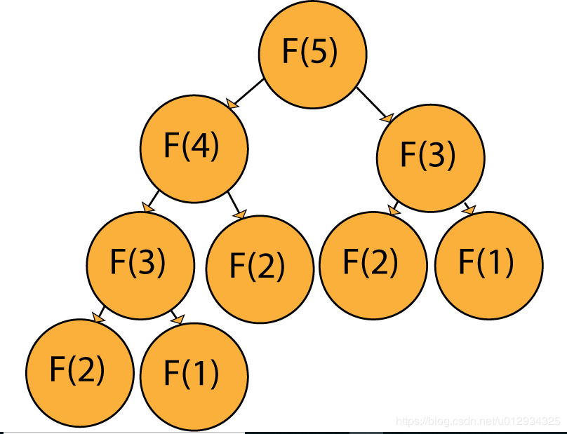
例如:如果我们想计算F(5),明显的我们需要计算F(3)和F(4)作为计算F(5)的先决条件。然而,为了计算F(4),我们需要计算F(3)和F(2),因此我们又需要计算F(2)和F(1)来得到F(3),其他的求解诸如此类。
这样的话就会导致很多重复的计算,这些重复计算本质上是冗余的,并且明显的减慢了算法的效率。为了解决这种问题,我们介绍动态规划。
在这种方法中,我们对解决方案进行建模,就像我们要递归地解决它一样,但我们从头开始解决它,记忆到达顶部采取的子问题(子步骤)的解决方案。
因此,对于Fibonacci序列,我们首先求解并记忆F(1)和F(2),然后使用两个记忆步骤计算F(3),依此类推。这意味着序列中每个单独元素的计算都是O(1),因为我们已经知道前两个元素。
当使用动态规划解决问题的时候,我们一般会采用下面三个步骤:
- 确定适用于所述问题的递归关系
- 初始化内存、数组、矩阵的初始值
- 确保当我们进行递归调用(可以访问子问题的答案)的时候它总是被提前解决。
遵循这些规则,让我们来看一下使用动态规划的算法的例子:
3. 贪心算法
下面来以这个为例子:
Given a rod of length n and an array that contains prices of all pieces of size smaller than n. Determine the maximum value obtainable by cutting up the rod and selling the pieces.
3.1. 对于没有经验的开发者可能会采取下面这种做法
这个问题实际上是为动态规划量身定做的,但是因为这是我们的第一个真实例子,让我们看看运行这些代码会遇到多少问题:
public class naiveSolution {
    static int getValue(int[] values, int length) {
        if (length <= 0)
            return 0;
        int tmpMax = -1;
        for (int i = 0; i < length; i++) {
            tmpMax = Math.max(tmpMax, values[i] + getValue(values, length - i - 1));
        }
        return tmpMax;
    }

    public static void main(String[] args) {
        int[] values = new int[]{3, 7, 1, 3, 9};
        int rodLength = values.length;

        System.out.println("Max rod value: " + getValue(values, rodLength));
    }
}
输出结果:
Max rod value: 17
该解决方案虽然正确,但效率非常低,递归调用的结果没有保存,所以每次有重叠解决方案时,糟糕的代码不得不去解决相同的子问题。
3.2.动态方法
利用上面相同的基本原理,添加记忆化并排除递归调用,我们得到以下实现:
public class dpSolution {
    static int getValue(int[] values, int rodLength) {
        int[] subSolutions = new int[rodLength + 1];

        for (int i = 1; i <= rodLength; i++) {
            int tmpMax = -1;
            for (int j = 0; j < i; j++)
                tmpMax = Math.max(tmpMax, values[j] + subSolutions[i - j - 1]);
            subSolutions[i] = tmpMax;
        }
        return subSolutions[rodLength];
    }

    public static void main(String[] args) {
        int[] values = new int[]{3, 7, 1, 3, 9};
        int rodLength = values.length;

        System.out.println("Max rod value: " + getValue(values, rodLength));
    }
}
输出结果:
Max rod value: 17
正如我们所看到的的,输出结果是一样的,所不同的是时间和空间复杂度。
通过从头开始解决子问题,我们消除了递归调用的需要,利用已解决给定问题的所有先前子问题的事实。
性能的提升
为了给出动态方法效率更高的观点的证据,让我们尝试使用30个值来运行该算法。 一种算法需要大约5.2秒来执行,而动态解决方法需要大约0.000095秒来执行。
4. 简化的背包问题
简化的背包问题是一个优化问题,没有一个解决方案。这个问题的问题是 - “解决方案是否存在?”:
Given a set of items, each with a weight w1, w2... determine the number of each item to put in a knapsack so that the total weight is less than or equal to a given limit K.
给定一组物品,每个物品的重量为w1,w2 ......确定放入背包中的每个物品的数量,以使总重量小于或等于给定的极限K
首先让我们把元素的所有权重存储在W数组中。接下来,假设有n个项目,我们将使用从1到n的数字枚举它们,因此第i个项目的权重为W [i]。我们将形成(n + 1)x(K + 1)维的矩阵M。M [x] [y]对应于背包问题的解决方案,但仅包括起始数组的前x个项,并且最大容量为y
例如
假设我们有3个元素,权重分别是w1=2kg,w2=3kg,w3=4kg。利用上面的方法,我们可以说M [1] [2]是一个有效的解决方案。
这意味着我们正在尝试用重量阵列中的第一个项目(w1)填充容量为2kg的背包。
在M [3] [5]中,我们尝试使用重量阵列的前3项(w1,w2,w3)填充容量为5kg的背包。
这不是一个有效的解决方案,因为我们过度拟合它。
4.1. 矩阵初始化
当初始化矩阵的时候有两点需要注意:
Does a solution exist for the given subproblem (M[x][y].exists) AND does the given solution include the latest item added to the array (M[x][y].includes).
给定子问题是否存在解(M [x] [y] .exists)并且给定解包括添加到数组的最新项(M [x] [y] .includes)。
因此,初始化矩阵是相当容易的,M[0][k].exists总是false,如果k>0,因为我们没有把任何物品放在带有k容量的背包里。
另一方面,M[0][0].exists = true,当k=0的时候,背包应该是空的,因此我们在里面没有放任何东西,这个是一个有效的解决方案。
此外,我们可以说M[k][0].exists = true,但是对于每个k来说 M[k][0].includes = false。
注意:仅仅因为对于给定的M [x] [y]存在解决方案,它并不一定意味着该特定组合是解决方案。
在M [10] [0]的情况下,存在一种解决方案 - 不包括10个元素中的任何一个。
这就是M [10] [0] .exists = true但M [10] [0] .includes = false的原因。
4.2.算法原则
接下来,让我们使用以下伪代码构造M [i] [k]的递归关系:
if (M[i-1][k].exists == True):
    M[i][k].exists = True
    M[i][k].includes = False
elif (k-W[i]>=0):
    if(M[i-1][k-W[i]].exists == true):
        M[i][k].exists = True
        M[i][k].includes = True
else:
    M[i][k].exists = False
因此,解决方案的要点是将子问题分为两种情况:
- 对于容量
k,当存在第一个i-1元素的解决方案 - 对于容量
k-W [i],当第一个i-1元素存在解决方案
第一种情况是不言自明的,我们已经有了问题的解决方案。
第二种情况是指了解第一个i-1元素的解决方案,但是容量只有一个第i个元素不满,这意味着我们可以添加一个第i个元素,并且我们有一个新的解决方案!
4.3. 实现
下面这何种实现方式,使得事情变得更加容易,我们创建了一个类Element来存储元素:
public class Element {
    private boolean exists;
    private boolean includes;

    public Element(boolean exists, boolean includes) {
        this.exists = exists;
        this.includes = includes;
    }

    public Element(boolean exists) {
        this.exists = exists;
        this.includes = false;
    }

    public boolean isExists() {
        return exists;
    }

    public void setExists(boolean exists) {
        this.exists = exists;
    }

    public boolean isIncludes() {
        return includes;
    }

    public void setIncludes(boolean includes) {
        this.includes = includes;
    }
}
接着,我们可以深入了解主要的类:
public class Knapsack {
    public static void main(String[] args) {
        Scanner scanner = new Scanner (System.in);

        System.out.println("Insert knapsack capacity:");
        int k = scanner.nextInt();

        System.out.println("Insert number of items:");
        int n = scanner.nextInt();

        System.out.println("Insert weights: ");
        int[] weights = new int[n + 1];

        for (int i = 1; i <= n; i++) {
            weights[i] = scanner.nextInt();
        }

        Element[][] elementMatrix = new Element[n + 1][k + 1];

        elementMatrix[0][0] = new Element(true);

        for (int i = 1; i <= k; i++) {
            elementMatrix[0][i] = new Element(false);
        }

        for (int i = 1; i <= n; i++) {
            for (int j = 0; j <= k; j++) {
                elementMatrix[i][j] = new Element(false);
                if (elementMatrix[i - 1][j].isExists()) {
                    elementMatrix[i][j].setExists(true);
                    elementMatrix[i][j].setIncludes(false);
                } else if (j >= weights[i]) {
                    if (elementMatrix[i - 1][j - weights[i]].isExists()) {
                        elementMatrix[i][j].setExists(true);
                        elementMatrix[i][j].setIncludes(true);
                    }
                }
            }
        }

        System.out.println(elementMatrix[n][k].isExists());
    }
}
唯一剩下的就是解决方案的重建,在上面的类中,我们知道解决方案是存在的,但是我们不知道它是什么。
为了重建,我们使用下面的代码:
List<Integer> solution = new ArrayList<>(n);

if (elementMatrix[n][k].isExists()) {
    int i = n;
    int j = k;
    while (j > 0 && i > 0) {
        if (elementMatrix[i][j].isIncludes()) {
            solution.add(i);
            j = j - weights[i];
        }
        i = i - 1;
    }
}

System.out.println("The elements with the following indexes are in the solution:\n" + (solution.toString()));
输出:
Insert knapsack capacity:
12
Insert number of items:
5
Insert weights:
9 7 4 10 3
true
The elements with the following indexes are in the solution:
[5, 1]
背包问题的一个简单变化是在没有价值优化的情况下填充背包,但现在每个单独项目的数量无限。
通过对现有代码进行简单调整,可以解决这种变化:
// Old code for simplified knapsack problem
else if (j >= weights[i]) {
    if (elementMatrix[i - 1][j - weights[i]].isExists()) {
        elementMatrix[i][j].setExists(true);
        elementMatrix[i][j].setIncludes(true);
    }
}

// New code, note that we're searching for a solution in the same
// row (i-th row), which means we're looking for a solution that
// already has some number of i-th elements (including 0) in it's solution
else if (j >= weights[i]) {
    if (elementMatrix[i][j - weights[i]].isExists()) {
        elementMatrix[i][j].setExists(true);
        elementMatrix[i][j].setIncludes(true);
    }
}
5. 传统的背包问题
利用以前的两种变体,现在让我们来看看传统的背包问题,看看它与简化版本的不同之处:
Given a set of items, each with a weight w1, w2... and a value v1, v2... determine the number of each item to include in a collection so that the total weight is less than or equal to a given limit k and the total value is as large as possible.
在简化版中,每个解决方案都同样出色。但是,现在我们有一个找到最佳解决方案的标准(也就是可能的最大值)。请记住,这次我们每个项目都有无限数量,因此项目可以在解决方案中多次出现。
在实现中,我们将使用旧的类Element,其中添加了私有字段value,用于存储给定子问题的最大可能值:
public class Element {
    private boolean exists;
    private boolean includes;
    private int value;
    // appropriate constructors, getters and setters
}
实现非常相似,唯一的区别是现在我们必须根据结果值选择最佳解决方案:
public static void main(String[] args) {
    // Same code as before with the addition of the values[] array
    System.out.println("Insert values: ");
    int[] values = new int[n + 1];

    for (int i=1; i <= n; i++) {
        values[i] = scanner.nextInt();
    }

    Element[][] elementMatrix = new Element[n + 1][k + 1];

    // A matrix that indicates how many newest objects are used
    // in the optimal solution.
    // Example: contains[5][10] indicates how many objects with
    // the weight of W[5] are contained in the optimal solution
    // for a knapsack of capacity K=10
    int[][] contains = new int[n + 1][k + 1];

    elementMatrix[0][0] = new Element(0);

    for (int i = 1; i <= n; i++) {
        elementMatrix[i][0] = new Element(0);
        contains[i][0] = 0;
    }

    for (int i = 1; i <= k; i++) {
        elementMatrix[0][i] = new Element(0);
        contains[0][i] = 0;
    }

    for (int i = 1; i <= n; i++) {
        for (int j = 0; j <= k; j++) {
            elementMatrix[i][j] = new Element(elementMatrix[i - 1][j].getValue());
            contains[i][j] = 0;

            elementMatrix[i][j].setIncludes(false);
            elementMatrix[i][j].setValue(M[i - 1][j].getValue());

            if (j >= weights[i]) {
                if ((elementMatrix[i][j - weights[i]].getValue() > 0 || j == weights[i])) {
                    if (elementMatrix[i][j - weights[i]].getValue() + values[i] > M[i][j].getValue()) {
                        elementMatrix[i][j].setIncludes(true);
                        elementMatrix[i][j].setValue(M[i][j - weights[i]].getValue() + values[i]);
                        contains[i][j] = contains[i][j - weights[i]] + 1;
                    }
                }
            }

            System.out.print(elementMatrix[i][j].getValue() + "/" + contains[i][j] + "  ");
        }

        System.out.println();
    }

    System.out.println("Value: " + elementMatrix[n][k].getValue());
}
输出:
Insert knapsack capacity:
12
Insert number of items:
5
Insert weights:
9 7 4 10 3
Insert values:
1 2 3 4 5
0/0  0/0  0/0  0/0  0/0  0/0  0/0  0/0  0/0  1/1  0/0  0/0  0/0
0/0  0/0  0/0  0/0  0/0  0/0  0/0  2/1  0/0  1/0  0/0  0/0  0/0
0/0  0/0  0/0  0/0  3/1  0/0  0/0  2/0  6/2  1/0  0/0  5/1  9/3
0/0  0/0  0/0  0/0  3/0  0/0  0/0  2/0  6/0  1/0  4/1  5/0  9/0
0/0  0/0  0/0  5/1  3/0  0/0  10/2  8/1  6/0  15/3  13/2  11/1  20/4
Value: 20
6. Levenshtein Distance
另一个使用动态规划的非常好的例子是Edit Distance或Levenshtein Distance。
Levenshtein Distance就是两个字符串A,B,我们需要使用原子操作将A转换为B:
- 字符串删除
- 字符串插入
- 字符替换(从技术上讲,它不止一个操作,但为了简单起见,我们称之为原子操作)
这个问题是通过有条理地解决起始字符串的子串的问题来处理的,逐渐增加子字符串的大小,直到它们等于起始字符串。
我们用于此问题的递归关系如下:
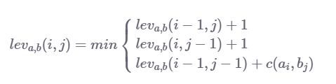
a == b则c(a,b)为0,如果a = = b则c(a,b)为1。
实现:
public class editDistance {
    public static void main(String[] args) {
        String s1, s2;
        Scanner scanner = new Scanner(System.in);
        System.out.println("Insert first string:");
        s1 = scanner.next();
        System.out.println("Insert second string:");
        s2 = scanner.next();

        int n, m;
        n = s1.length();
        m = s2.length();

        // Matrix of substring edit distances
        // example: distance[a][b] is the edit distance
        // of the first a letters of s1 and b letters of s2
        int[][] distance = new int[n + 1][m + 1];

        // Matrix initialization:
        // If we want to turn any string into an empty string
        // the fastest way no doubt is to just delete
        // every letter individually.
        // The same principle applies if we have to turn an empty string
        // into a non empty string, we just add appropriate letters
        // until the strings are equal.
        for (int i = 0; i <= n; i++) {
            distance[i][0] = i;
        }
        for (int j = 0; j <= n; j++) {
            distance[0][j] = j;
        }

        // Variables for storing potential values of current edit distance
        int e1, e2, e3, min;

        for (int i = 1; i <= n; i++) {
            for (int j = 1; j <= m; j++) {
                e1 = distance[i - 1][j] + 1;
                e2 = distance[i][j - 1] + 1;
                if (s1.charAt(i - 1) == s2.charAt(j - 1)) {
                    e3 = distance[i - 1][j - 1];
                } else {
                    e3 = distance[i - 1][j - 1] + 1;
                }
                min = Math.min(e1, e2);
                min = Math.min(min, e3);
                distance[i][j] = min;
            }

        }

        System.out.println("Edit distance of s1 and s2 is: " + distance[n][m]);
    }
}
输出:
Insert first string:
man
Insert second string:
machine
Edit distance of s1 and s2 is: 3
如果你想了解更多关于Levenshtein Distance的解决方案,我们在另外的一篇文章中用python实现了 Levenshtein Distance and Text Similarity in Python,
使用这个逻辑,我们可以将许多字符串比较算法归结为简单的递归关系,它使用Levenshtein Distance的基本公式
7. 最长共同子序列(LCS)
这个问题描述如下:
Given two sequences, find the length of the longest subsequence present in both of them. A subsequence is a sequence that appears in the same relative order, but not necessarily contiguous.
给定两个序列,找到两个序列中存在的最长子序列的长度。子序列是以相同的相对顺序出现的序列,但不一定是连续的.
阐明:
如果我们有两个字符串s1="MICE"和s2="MINCE",最长的共同子序列是MI或者CE。但是,最长的公共子序列将是“MICE”,因为结果子序列的元素不必是连续的顺序。
递归关系与一般逻辑:
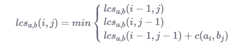
Levenshtein distance和LCS之间只有微小的差别,特别是移动成本。
在LCS中,我们没有字符插入和字符删除的成本,这意味着我们只计算字符替换(对角线移动)的成本,如果两个当前字符串字符a [i]和b [j] 是相同的,则成本为1。
LCS的最终成本是2个字符串的最长子序列的长度,这正是我们所需要的。
Using this logic, we can boil down a lot of string comparison algorithms to simple recurrence relations which utilize the base formula of the Levenshtein distance
使用这个逻辑,我们可以将许多字符串比较算法归结为简单的递归关系,它使用Levenshtein distance的基本公式。
实现:
public class LCS {
    public static void main(String[] args) {
        String s1 = new String("Hillfinger");
        String s2 = new String("Hilfiger");
        int n = s1.length();
        int m = s2.length();
        int[][] solutionMatrix = new int[n+1][m+1];
        for (int i = 0; i < n; i++) {
            solutionMatrix[i][0] = 0;
        }
        for (int i = 0; i < m; i++) {
            solutionMatrix[0][i] = 0;
        }

        for (int i = 1; i <= n; i++) {
            for (int j = 1; j <= m; j++) {
                int max1, max2, max3;
                max1 = solutionMatrix[i - 1][j];
                max2 = solutionMatrix[i][j - 1];
                if (s1.charAt(i - 1) == s2.charAt(j - 1)) {
                    max3 = solutionMatrix[i - 1][j - 1] + 1;
                } else {
                    max3 = solutionMatrix[i - 1][j - 1];
                }
                int tmp = Math.max(max1, max2);
                solutionMatrix[i][j] = Math.max(tmp, max3);
            }
        }

        System.out.println("Length of longest continuous subsequence: " + solutionMatrix[n][m]);
    }
}
输出:
Length of longest continuous subsequence: 8
8.利用动态规划的其他问题
利用动态规划可以解决很多问题,下面列举了一些:
- 分区问题:给定一组整数,找出它是否可以分成两个具有相等和的子集
- 子集和问题:给你一个正整数的数组及元素还有一个合计值,是否在数组中存在一个子集的的元素之和等于合计值。
- 硬币变化问题:鉴于给定面额的硬币无限供应,找到获得所需变化的不同方式的总数
- k变量线性方程的所有可能的解:给定k个变量的线性方程,计算它的可能解的总数
- 找到醉汉不会从悬崖上掉下来的概率:给定一个线性空间代表距离悬崖的距离,让你知道酒鬼从悬崖起始的距离,以及他向悬崖p前进并远离悬崖1-p的倾向,计算出他的生存概率
9.结论
动态编程是一种工具,可以节省大量的计算时间,以换取更大的空间复杂性,这在很大程度上取决于您正在处理的系统类型,如果CPU时间很宝贵,您选择耗费内存的解决方案,另一方面,如果您的内存有限,则选择更耗时的解决方案。
作者: Vladimir Batoćanin
译者:lee