

题图来自:github
本文主要演示了在CIFAR-10数据集上进行图像识别。
其中有大段之前教程的文字及代码,如果看过的朋友可以快速翻阅。01 - 简单线性模型 | 02 - 卷积神经网络 | 03 - PrettyTensor | 04 - 保存& 恢复
05 - 集成学习
by Magnus Erik Hvass Pedersen / GitHub / Videos on YouTube
中文翻译 thrillerist / Github
简介
这篇教程介绍了如何创建一个在CIRAR-10数据集上进行图像分类的卷积神经网络。同时也说明了在训练和测试时如何使用不同的网络。
本文基于上一篇教程,你需要了解基本的TensorFlow和附加包Pretty Tensor。其中大量代码和文字与之前教程相似,如果你已经看过可以快速地浏览本文。
流程图
下面的图表直接显示了之后实现的卷积神经网络中数据的传递。首先有一个扭曲(distorts)输入图像的预处理层,用来人为地扩大训练集。接着有两个卷积层,两个全连接层和一个softmax分类层。在后面会有更大的图示来显示权重和卷积层的输出,教程 #02 有卷积如何工作的更多细节。
在这种情况下图像是误分类的。图像上有一只狗,但神经网络不确定它是狗还是猫,认为更有可能是猫。
from IPython.display import Image
Image('images/06_network_flowchart.png')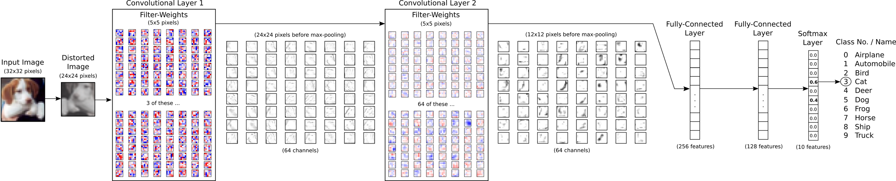
导入
%matplotlib inline
import matplotlib.pyplot as plt
import tensorflow as tf
import numpy as np
from sklearn.metrics import confusion_matrix
import time
from datetime import timedelta
import math
import os

# Use PrettyTensor to simplify Neural Network construction.
import prettytensor as pt
使用Python3.5.2(Anaconda)开发,TensorFlow版本是:
tf.__version__'0.12.0-rc0'
PrettyTensor 版本:
pt.__version__'0.7.1'
载入数据
import cifar10设置电脑上保存数据集的路径。
# cifar10.data_path = "data/CIFAR-10/"CIFAR-10数据集大概有163MB,如果给定路径没有找到文件的话,将会自动下载。
cifar10.maybe_download_and_extract()Data has apparently already been downloaded and unpacked.
载入分类名称。
class_names = cifar10.load_class_names()
class_names
Loading data: data/CIFAR-10/cifar-10-batches-py/batches.meta
['airplane',
'automobile',
'bird',
'cat',
'deer',
'dog',
'frog',
'horse',
'ship',
'truck']
载入训练集。这个函数返回图像、整形分类号码、以及用One-Hot编码的分类号数组,称为标签。
images_train, cls_train, labels_train = cifar10.load_training_data()Loading data: data/CIFAR-10/cifar-10-batches-py/data_batch_1
Loading data: data/CIFAR-10/cifar-10-batches-py/data_batch_2
Loading data: data/CIFAR-10/cifar-10-batches-py/data_batch_3
Loading data: data/CIFAR-10/cifar-10-batches-py/data_batch_4
Loading data: data/CIFAR-10/cifar-10-batches-py/data_batch_5
载入测试集。
images_test, cls_test, labels_test = cifar10.load_test_data()Loading data: data/CIFAR-10/cifar-10-batches-py/test_batch
现在已经载入了CIFAR-10数据集,它包含60,000张图像以及相关的标签(图像的分类)。数据集被分为两个独立的子集,即训练集和测试集。
print("Size of:")
print("- Training-set:\t\t{}".format(len(images_train)))
print("- Test-set:\t\t{}".format(len(images_test)))
Size of:
- Training-set: 50000
- Test-set: 10000
数据维度
下面的代码中多次用到数据维度。cirfa10模块中已经定义好了这些,因此我们只需要import进来。
from cifar10 import img_size, num_channels, num_classes图像是32 x 32像素的,但我们将图像裁剪至24 x 24像素。
img_size_cropped = 24用来绘制图片的帮助函数
这个函数用来在3x3的栅格中画9张图像,然后在每张图像下面写出真实类别和预测类别。
def plot_images(images, cls_true, cls_pred=None, smooth=True):

    assert len(images) == len(cls_true) == 9

    # Create figure with sub-plots.
    fig, axes = plt.subplots(3, 3)

    # Adjust vertical spacing if we need to print ensemble and best-net.
    if cls_pred is None:
        hspace = 0.3
    else:
        hspace = 0.6
    fig.subplots_adjust(hspace=hspace, wspace=0.3)

    for i, ax in enumerate(axes.flat):
        # Interpolation type.
        if smooth:
            interpolation = 'spline16'
        else:
            interpolation = 'nearest'

        # Plot image.
        ax.imshow(images[i, :, :, :],
                  interpolation=interpolation)

        # Name of the true class.
        cls_true_name = class_names[cls_true[i]]

        # Show true and predicted classes.
        if cls_pred is None:
            xlabel = "True: {0}".format(cls_true_name)
        else:
            # Name of the predicted class.
            cls_pred_name = class_names[cls_pred[i]]

            xlabel = "True: {0}\nPred: {1}".format(cls_true_name, cls_pred_name)

        # Show the classes as the label on the x-axis.
        ax.set_xlabel(xlabel)

        # Remove ticks from the plot.
        ax.set_xticks([])
        ax.set_yticks([])

    # Ensure the plot is shown correctly with multiple plots
    # in a single Notebook cell.
    plt.show()
绘制几张图像来看看数据是否正确
# Get the first images from the test-set.
images = images_test[0:9]

# Get the true classes for those images.
cls_true = cls_test[0:9]

# Plot the images and labels using our helper-function above.
plot_images(images=images, cls_true=cls_true, smooth=False)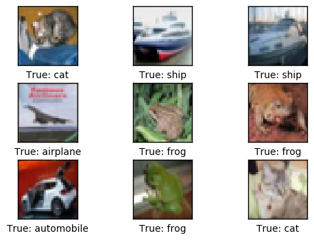
上面像素化的图像是神经网络的输入。如果我们对图像进行平滑处理,可能更易于人眼识别。
plot_images(images=images, cls_true=cls_true, smooth=True)
TensorFlow图
TensorFlow的全部目的就是使用一个称之为计算图(computational graph)的东西,它会比直接在Python中进行相同计算量要高效得多。TensorFlow比Numpy更高效,因为TensorFlow了解整个需要运行的计算图,然而Numpy只知道某个时间点上唯一的数学运算。
TensorFlow也能够自动地计算需要优化的变量的梯度,使得模型有更好的表现。这是由于图是简单数学表达式的结合,因此整个图的梯度可以用链式法则推导出来。
TensorFlow还能利用多核CPU和GPU,Google也为TensorFlow制造了称为TPUs(Tensor Processing Units)的特殊芯片,它比GPU更快。
一个TensorFlow图由下面几个部分组成,后面会详细描述:
- 占位符变量(Placeholder)用来改变图的输入。
- 模型变量(Model)将会被优化,使得模型表现得更好。
- 模型本质上就是一些数学函数,它根据Placeholder和模型的输入变量来计算一些输出。
- 一个cost度量用来指导变量的优化。
- 一个优化策略会更新模型的变量。
另外,TensorFlow图也包含了一些调试状态,比如用TensorBoard打印log数据,本教程不涉及这些。
占位符 (Placeholder)变量
Placeholder是作为图的输入,我们每次运行图的时候都可能改变它们。将这个过程称为feeding placeholder变量,后面将会描述这个。
首先我们为输入图像定义placeholder变量。这让我们可以改变输入到TensorFlow图中的图像。这也是一个张量(tensor),代表一个多维向量或矩阵。数据类型设置为float32,形状设为[None, img_size, img_size, num_channels]代表tensor可能保存着任意数量的图像,每张图像宽高都为img_size,有num_channels个颜色通道。
x = tf.placeholder(tf.float32, shape=[None, img_size, img_size, num_channels], name='x')接下来我们为输入变量x中的图像所对应的真实标签定义placeholder变量。变量的形状是[None, num_classes],这代表着它保存了任意数量的标签,每个标签是长度为num_classes的向量,本例中长度为10。
y_true = tf.placeholder(tf.float32, shape=[None, num_classes], name='y_true')我们也可以为class-number提供一个placeholder,但这里用argmax来计算它。这里只是TensorFlow中的一些操作,没有执行什么运算。
y_true_cls = tf.argmax(y_true, dimension=1)预处理的帮助函数
下面的帮助函数创建了用来预处理输入图像的TensorFlow计算图。这里并未执行计算,函数只是给TensorFlow计算图添加了节点。
神经网络在训练和测试阶段的预处理方法不同:
对于训练来说,输入图像是随机裁剪、水平翻转的,并且用随机值来调整色调、对比度和饱和度。这样就创建了原始输入图像的随机变体,人为地扩充了训练集。后面会显示一些扭曲过的图像样本。
对于测试,输入图像根据中心裁剪,其他不作调整。
def pre_process_image(image, training):
    # This function takes a single image as input,
    # and a boolean whether to build the training or testing graph.

    if training:
        # For training, add the following to the TensorFlow graph.

        # Randomly crop the input image.
        image = tf.random_crop(image, size=[img_size_cropped, img_size_cropped, num_channels])

        # Randomly flip the image horizontally.
        image = tf.image.random_flip_left_right(image)

        # Randomly adjust hue, contrast and saturation.
        image = tf.image.random_hue(image, max_delta=0.05)
        image = tf.image.random_contrast(image, lower=0.3, upper=1.0)
        image = tf.image.random_brightness(image, max_delta=0.2)
        image = tf.image.random_saturation(image, lower=0.0, upper=2.0)

        # Some of these functions may overflow and result in pixel
        # values beyond the [0, 1] range. It is unclear from the
        # documentation of TensorFlow 0.10.0rc0 whether this is
        # intended. A simple solution is to limit the range.

        # Limit the image pixels between [0, 1] in case of overflow.
        image = tf.minimum(image, 1.0)
        image = tf.maximum(image, 0.0)
    else:
        # For training, add the following to the TensorFlow graph.

        # Crop the input image around the centre so it is the same
        # size as images that are randomly cropped during training.
        image = tf.image.resize_image_with_crop_or_pad(image,
                                                       target_height=img_size_cropped,
                                                       target_width=img_size_cropped)

    return image
下面函数中,输入batch中每张图像都调用以上函数。
def pre_process(images, training):
    # Use TensorFlow to loop over all the input images and call
    # the function above which takes a single image as input.
    images = tf.map_fn(lambda image: pre_process_image(image, training), images)

    return images
为了绘制扭曲过的图像,我们为TensorFlow创建预处理graph,后面将会运行它。
distorted_images = pre_process(images=x, training=True)创建主要处理程序的帮助函数
下面的帮助函数创建了卷积神经网络的主要部分。这里使用之前教程描述过的Pretty Tensor。
def main_network(images, training):
    # Wrap the input images as a Pretty Tensor object.
    x_pretty = pt.wrap(images)

    # Pretty Tensor uses special numbers to distinguish between
    # the training and testing phases.
    if training:
        phase = pt.Phase.train
    else:
        phase = pt.Phase.infer

    # Create the convolutional neural network using Pretty Tensor.
    # It is very similar to the previous tutorials, except
    # the use of so-called batch-normalization in the first layer.
    with pt.defaults_scope(activation_fn=tf.nn.relu, phase=phase):
        y_pred, loss = x_pretty.\
            conv2d(kernel=5, depth=64, name='layer_conv1', batch_normalize=True).\
            max_pool(kernel=2, stride=2).\
            conv2d(kernel=5, depth=64, name='layer_conv2').\
            max_pool(kernel=2, stride=2).\
            flatten().\
            fully_connected(size=256, name='layer_fc1').\
            fully_connected(size=128, name='layer_fc2').\
            softmax_classifier(num_classes=num_classes, labels=y_true)

    return y_pred, loss
创建神经网络的帮助函数
下面的帮助函数创建了整个神经网络,包含上面定义的预处理以及主要处理模块。
注意,神经网络被编码到'network'变量作用域中。因为我们实际上在TensorFlow图中创建了两个神经网络。像这样指定一个变量作用域,可以在两个神经网络中复用变量,因此训练网络优化过的变量可以在测试网络中复用。
def create_network(training):
    # Wrap the neural network in the scope named 'network'.
    # Create new variables during training, and re-use during testing.
    with tf.variable_scope('network', reuse=not training):
        # Just rename the input placeholder variable for convenience.
        images = x

        # Create TensorFlow graph for pre-processing.
        images = pre_process(images=images, training=training)

        # Create TensorFlow graph for the main processing.
        y_pred, loss = main_network(images=images, training=training)

    return y_pred, loss
为训练阶段创建神经网络
首先创建一个保存当前优化迭代次数的TensorFlow变量。在之前的教程中,是使用一个Python变量,但本教程中,我们想用checkpoints中的其他TensorFlow变量来保存。
trainable=False表示TensorFlow不会优化此变量。
global_step = tf.Variable(initial_value=0,
                          name='global_step', trainable=False)
创建训练用的神经网络。函数 create_network()返回y_pred和loss,但在训练时我们只需用到loss函数。
_, loss = create_network(training=True)创建最小化loss函数的优化器。同时将global_step传给优化器,这样每次迭代它都减一。
optimizer = tf.train.AdamOptimizer(learning_rate=1e-4).minimize(loss, global_step=global_step)创建测试阶段的神经网络
现在创建测试阶段的神经网络。 同样的,create_network() 返回输入图像的预测标签 y_pred,优化过程也用到 loss函数。测试时我们只需要y_pred。
y_pred, _ = create_network(training=False)然后我们计算预测类别号的整形数字。网络的输出y_pred是一个10个元素的数组。类别号是数组中最大元素的索引。
y_pred_cls = tf.argmax(y_pred, dimension=1)然后创建一个布尔向量,用来告诉我们每张图片的真实类别是否与预测类别相同。
correct_prediction = tf.equal(y_pred_cls, y_true_cls)上面的计算先将布尔值向量类型转换成浮点型向量,这样子False就变成0,True变成1,然后计算这些值的平均数,以此来计算分类的准确率。
accuracy = tf.reduce_mean(tf.cast(correct_prediction, tf.float32))Saver
为了保存神经网络的变量(这样不必再次训练网络就能重载),我们创建一个称为Saver-object的对象,它用来保存及恢复TensorFlow图的所有变量。在这里并未保存什么东西,(保存操作)在后面的optimize()函数中完成。
saver = tf.train.Saver()获取权重
下面,我们要绘制神经网络的权重。当使用Pretty Tensor来创建网络时,层的所有变量都是由Pretty Tensoe间接创建的。因此我们要从TensorFlow中获取变量。
我们用layer_conv1 和 layer_conv2代表两个卷积层。这也叫变量作用域(不要与上面描述的defaults_scope混淆了)。PrettyTensor会自动给它为每个层创建的变量命名,因此我们可以通过层的作用域名称和变量名来取得某一层的权重。
函数实现有点笨拙,因为我们不得不用TensorFlow函数get_variable(),它是设计给其他用途的,创建新的变量或重用现有变量。创建下面的帮助函数很简单。
def get_weights_variable(layer_name):
    # Retrieve an existing variable named 'weights' in the scope
    # with the given layer_name.
    # This is awkward because the TensorFlow function was
    # really intended for another purpose.

    with tf.variable_scope("network/" + layer_name, reuse=True):
        variable = tf.get_variable('weights')

    return variable
借助这个帮助函数我们可以获取变量。这些是TensorFlow的objects。你需要类似的操作来获取变量的内容: contents = session.run(weights_conv1) ,下面会提到这个。
weights_conv1 = get_weights_variable(layer_name='layer_conv1')
weights_conv2 = get_weights_variable(layer_name='layer_conv2')
获取layer的输出
同样的,我们还需要获取卷积层的输出。这个函数与上面获取权重的函数有所不同。这里我们找回卷积层输出的最后一个张量。
def get_layer_output(layer_name):
    # The name of the last operation of the convolutional layer.
    # This assumes you are using Relu as the activation-function.
    tensor_name = "network/" + layer_name + "/Relu:0"

    # Get the tensor with this name.
    tensor = tf.get_default_graph().get_tensor_by_name(tensor_name)

    return tensor
取得卷积层的输出以便之后绘制。
output_conv1 = get_layer_output(layer_name='layer_conv1')
output_conv2 = get_layer_output(layer_name='layer_conv2')
运行TensorFlow
创建TensorFlow会话(session)
一旦创建了TensorFlow图,我们需要创建一个TensorFlow会话,用来运行图。
session = tf.Session()初始化或恢复变量
训练神经网络会花上很长时间,特别是当你没有GPU的时候。因此我们在训练时保存checkpoints,这样就能在其他时间继续训练(比如晚上),以后也可以不用训练神经网络就用这些来分析结果。
如果你想重新训练神经网络,就需要先删掉这些checkpoints。
这是用来保存checkpoints的文件夹。
save_dir = 'checkpoints/'如果文件夹不存在则创建。
if not os.path.exists(save_dir):
    os.makedirs(save_dir)
这是checkpoints的基本文件名,TensorFlow会在后面添加迭代次数等。
save_path = os.path.join(save_dir, 'cifar10_cnn')试着载入最新的checkpoint。如果checkpoint不存在或改变了TensorFlow图的话,可能会失败并抛出异常。
try:
    print("Trying to restore last checkpoint ...")

    # Use TensorFlow to find the latest checkpoint - if any.
    last_chk_path = tf.train.latest_checkpoint(checkpoint_dir=save_dir)

    # Try and load the data in the checkpoint.
    saver.restore(session, save_path=last_chk_path)

    # If we get to this point, the checkpoint was successfully loaded.
    print("Restored checkpoint from:", last_chk_path)
except:
    # If the above failed for some reason, simply
    # initialize all the variables for the TensorFlow graph.
    print("Failed to restore checkpoint. Initializing variables instead.")
    session.run(tf.global_variables_initializer())
Trying to restore last checkpoint ...
Restored checkpoint from: checkpoints/cifar10_cnn-150000创建随机训练batch的帮助函数
在训练集中有50,000张图。用这些图像计算模型的梯度会花很多时间。因此,在优化器的每次迭代里只用到了一小部分的图像。
如果内存耗尽导致电脑死机或变得很慢,你应该试着减少这些数量,但同时可能还需要更优化的迭代。
train_batch_size = 64函数从训练集中挑选一个随机的training-batch。
def random_batch():
    # Number of images in the training-set.
    num_images = len(images_train)

    # Create a random index.
    idx = np.random.choice(num_images,
                           size=train_batch_size,
                           replace=False)

    # Use the random index to select random images and labels.
    x_batch = images_train[idx, :, :, :]
    y_batch = labels_train[idx, :]

    return x_batch, y_batch
执行优化迭代的帮助函数
函数用来执行一定数量的优化迭代,以此来逐渐改善网络层的变量。在每次迭代中,会从训练集中选择新的一批数据,然后TensorFlow在这些训练样本上执行优化。每100次迭代会打印出进度。每1000次迭代后会保存一个checkpoint,最后一次迭代完毕也会保存。
def optimize(num_iterations):
    # Start-time used for printing time-usage below.
    start_time = time.time()

    for i in range(num_iterations):
        # Get a batch of training examples.
        # x_batch now holds a batch of images and
        # y_true_batch are the true labels for those images.
        x_batch, y_true_batch = random_batch()

        # Put the batch into a dict with the proper names
        # for placeholder variables in the TensorFlow graph.
        feed_dict_train = {x: x_batch,
                           y_true: y_true_batch}

        # Run the optimizer using this batch of training data.
        # TensorFlow assigns the variables in feed_dict_train
        # to the placeholder variables and then runs the optimizer.
        # We also want to retrieve the global_step counter.
        i_global, _ = session.run([global_step, optimizer],
                                  feed_dict=feed_dict_train)

        # Print status to screen every 100 iterations (and last).
        if (i_global % 100 == 0) or (i == num_iterations - 1):
            # Calculate the accuracy on the training-batch.
            batch_acc = session.run(accuracy,
                                    feed_dict=feed_dict_train)

            # Print status.
            msg = "Global Step: {0:>6}, Training Batch Accuracy: {1:>6.1%}"
            print(msg.format(i_global, batch_acc))

        # Save a checkpoint to disk every 1000 iterations (and last).
        if (i_global % 1000 == 0) or (i == num_iterations - 1):
            # Save all variables of the TensorFlow graph to a
            # checkpoint. Append the global_step counter
            # to the filename so we save the last several checkpoints.
            saver.save(session,
                       save_path=save_path,
                       global_step=global_step)

            print("Saved checkpoint.")

    # Ending time.
    end_time = time.time()

    # Difference between start and end-times.
    time_dif = end_time - start_time

    # Print the time-usage.
    print("Time usage: " + str(timedelta(seconds=int(round(time_dif)))))
用来绘制错误样本的帮助函数
函数用来绘制测试集中被误分类的样本。
def plot_example_errors(cls_pred, correct):
    # This function is called from print_test_accuracy() below.

    # cls_pred is an array of the predicted class-number for
    # all images in the test-set.

    # correct is a boolean array whether the predicted class
    # is equal to the true class for each image in the test-set.

    # Negate the boolean array.
    incorrect = (correct == False)

    # Get the images from the test-set that have been
    # incorrectly classified.
    images = images_test[incorrect]

    # Get the predicted classes for those images.
    cls_pred = cls_pred[incorrect]

    # Get the true classes for those images.
    cls_true = cls_test[incorrect]

    # Plot the first 9 images.
    plot_images(images=images[0:9],
                cls_true=cls_true[0:9],
                cls_pred=cls_pred[0:9])
绘制混淆(confusion)矩阵的帮助函数
def plot_confusion_matrix(cls_pred):
    # This is called from print_test_accuracy() below.

    # cls_pred is an array of the predicted class-number for
    # all images in the test-set.

    # Get the confusion matrix using sklearn.
    cm = confusion_matrix(y_true=cls_test,  # True class for test-set.
                          y_pred=cls_pred)  # Predicted class.

    # Print the confusion matrix as text.
    for i in range(num_classes):
        # Append the class-name to each line.
        class_name = "({}) {}".format(i, class_names[i])
        print(cm[i, :], class_name)

    # Print the class-numbers for easy reference.
    class_numbers = [" ({0})".format(i) for i in range(num_classes)]
    print("".join(class_numbers))
计算分类的帮助函数
这个函数用来计算图像的预测类别,同时返回一个代表每张图像分类是否正确的布尔数组。
由于计算可能会耗费太多内存,就分批处理。如果你的电脑死机了,试着降低batch-size。
# Split the data-set in batches of this size to limit RAM usage.
batch_size = 256

def predict_cls(images, labels, cls_true):
    # Number of images.
    num_images = len(images)

    # Allocate an array for the predicted classes which
    # will be calculated in batches and filled into this array.
    cls_pred = np.zeros(shape=num_images, dtype=np.int)

    # Now calculate the predicted classes for the batches.
    # We will just iterate through all the batches.
    # There might be a more clever and Pythonic way of doing this.

    # The starting index for the next batch is denoted i.
    i = 0

    while i < num_images:
        # The ending index for the next batch is denoted j.
        j = min(i + batch_size, num_images)

        # Create a feed-dict with the images and labels
        # between index i and j.
        feed_dict = {x: images[i:j, :],
                     y_true: labels[i:j, :]}

        # Calculate the predicted class using TensorFlow.
        cls_pred[i:j] = session.run(y_pred_cls, feed_dict=feed_dict)

        # Set the start-index for the next batch to the
        # end-index of the current batch.
        i = j

    # Create a boolean array whether each image is correctly classified.
    correct = (cls_true == cls_pred)

    return correct, cls_pred
计算测试集的预测类别。
def predict_cls_test():
    return predict_cls(images = images_test,
                       labels = labels_test,
                       cls_true = cls_test)
计算分类准确率的帮助函数
这个函数计算了给定布尔数组的分类准确率,布尔数组表示每张图像是否被正确分类。比如, cls_accuracy([True, True, False, False, False]) = 2/5 = 0.4。这个函数也返回了正确分类的数量。
def classification_accuracy(correct):
    # When averaging a boolean array, False means 0 and True means 1.
    # So we are calculating: number of True / len(correct) which is
    # the same as the classification accuracy.

    # Return the classification accuracy
    # and the number of correct classifications.
    return correct.mean(), correct.sum()
展示性能的帮助函数
函数用来打印测试集上的分类准确率。
为测试集上的所有图片计算分类会花费一段时间,因此我们直接从这个函数里调用上面的函数,这样就不用每个函数都重新计算分类。
def print_test_accuracy(show_example_errors=False,
                        show_confusion_matrix=False):

    # For all the images in the test-set,
    # calculate the predicted classes and whether they are correct.
    correct, cls_pred = predict_cls_test()

    # Classification accuracy and the number of correct classifications.
    acc, num_correct = classification_accuracy(correct)

    # Number of images being classified.
    num_images = len(correct)

    # Print the accuracy.
    msg = "Accuracy on Test-Set: {0:.1%} ({1} / {2})"
    print(msg.format(acc, num_correct, num_images))

    # Plot some examples of mis-classifications, if desired.
    if show_example_errors:
        print("Example errors:")
        plot_example_errors(cls_pred=cls_pred, correct=correct)

    # Plot the confusion matrix, if desired.
    if show_confusion_matrix:
        print("Confusion Matrix:")
        plot_confusion_matrix(cls_pred=cls_pred)
绘制卷积权重的帮助函数
def plot_conv_weights(weights, input_channel=0):
    # Assume weights are TensorFlow ops for 4-dim variables
    # e.g. weights_conv1 or weights_conv2.

    # Retrieve the values of the weight-variables from TensorFlow.
    # A feed-dict is not necessary because nothing is calculated.
    w = session.run(weights)

    # Print statistics for the weights.
    print("Min:  {0:.5f}, Max:   {1:.5f}".format(w.min(), w.max()))
    print("Mean: {0:.5f}, Stdev: {1:.5f}".format(w.mean(), w.std()))

    # Get the lowest and highest values for the weights.
    # This is used to correct the colour intensity across
    # the images so they can be compared with each other.
    w_min = np.min(w)
    w_max = np.max(w)
    abs_max = max(abs(w_min), abs(w_max))

    # Number of filters used in the conv. layer.
    num_filters = w.shape[3]

    # Number of grids to plot.
    # Rounded-up, square-root of the number of filters.
    num_grids = math.ceil(math.sqrt(num_filters))

    # Create figure with a grid of sub-plots.
    fig, axes = plt.subplots(num_grids, num_grids)

    # Plot all the filter-weights.
    for i, ax in enumerate(axes.flat):
        # Only plot the valid filter-weights.
        if i<num_filters:
            # Get the weights for the i'th filter of the input channel.
            # The format of this 4-dim tensor is determined by the
            # TensorFlow API. See Tutorial #02 for more details.
            img = w[:, :, input_channel, i]

            # Plot image.
            ax.imshow(img, vmin=-abs_max, vmax=abs_max,
                      interpolation='nearest', cmap='seismic')

        # Remove ticks from the plot.
        ax.set_xticks([])
        ax.set_yticks([])

    # Ensure the plot is shown correctly with multiple plots
    # in a single Notebook cell.
    plt.show()
绘制卷积层输出的帮助函数
def plot_layer_output(layer_output, image):
    # Assume layer_output is a 4-dim tensor
    # e.g. output_conv1 or output_conv2.

    # Create a feed-dict which holds the single input image.
    # Note that TensorFlow needs a list of images,
    # so we just create a list with this one image.
    feed_dict = {x: [image]}

    # Retrieve the output of the layer after inputting this image.
    values = session.run(layer_output, feed_dict=feed_dict)

    # Get the lowest and highest values.
    # This is used to correct the colour intensity across
    # the images so they can be compared with each other.
    values_min = np.min(values)
    values_max = np.max(values)

    # Number of image channels output by the conv. layer.
    num_images = values.shape[3]

    # Number of grid-cells to plot.
    # Rounded-up, square-root of the number of filters.
    num_grids = math.ceil(math.sqrt(num_images))

    # Create figure with a grid of sub-plots.
    fig, axes = plt.subplots(num_grids, num_grids)

    # Plot all the filter-weights.
    for i, ax in enumerate(axes.flat):
        # Only plot the valid image-channels.
        if i<num_images:
            # Get the images for the i'th output channel.
            img = values[0, :, :, i]

            # Plot image.
            ax.imshow(img, vmin=values_min, vmax=values_max,
                      interpolation='nearest', cmap='binary')

        # Remove ticks from the plot.
        ax.set_xticks([])
        ax.set_yticks([])

    # Ensure the plot is shown correctly with multiple plots
    # in a single Notebook cell.
    plt.show()
输入图像变体的样本
为了人为地增加训练用的图像数量,神经网络预处理获取输入图像的随机变体。这让神经网络在识别和分类图像时更加灵活。
这是用来绘制输入图像变体的帮助函数。
def plot_distorted_image(image, cls_true):
    # Repeat the input image 9 times.
    image_duplicates = np.repeat(image[np.newaxis, :, :, :], 9, axis=0)

    # Create a feed-dict for TensorFlow.
    feed_dict = {x: image_duplicates}

    # Calculate only the pre-processing of the TensorFlow graph
    # which distorts the images in the feed-dict.
    result = session.run(distorted_images, feed_dict=feed_dict)

    # Plot the images.
    plot_images(images=result, cls_true=np.repeat(cls_true, 9))
帮助函数获取测试集图像以及它的分类号。
def get_test_image(i):
    return images_test[i, :, :, :], cls_test[i]
从测试集中取一张图像以及它的真实类别。
img, cls = get_test_image(16)画出图像的9张随机变体。如果你重新运行代码,可能会得到不太一样的结果。
plot_distorted_image(img, cls)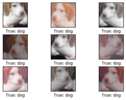
执行优化
我的笔记本电脑是4核的,每个2GHz。电脑带有一个GPU,但对TensorFlow来说不太快,因此只用了CPU。在电脑上迭代10,000次大概花了1个小时。本教程中我执行了150,000次优化迭代,共花了15个小时。我让它在夜里以及白天的几个时间段运行。
由于我们在优化过程中保存了checkpoints,重新运行代码时会载入最后的那个checkpoint,所以可以先停止,等晚点再继续执行优化。
if False:
    optimize(num_iterations=1000)
结果
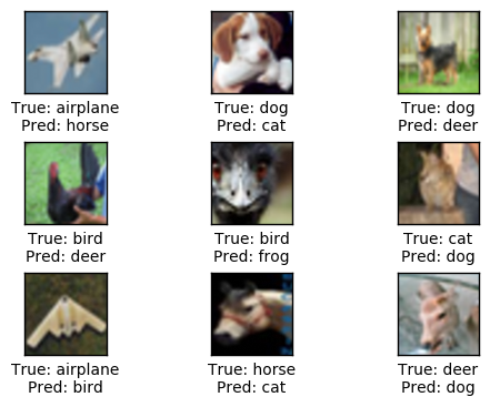
在150,000次优化迭代之后,测试集上的分类准确率大约79%-80%。下面画出了一些误分类的图像。其中有一些即使人眼也很难分辨出来,也有一些是合乎情理的错误,比如大型车和卡车,猫与狗,但有些错误就有点奇怪了。
print_test_accuracy(show_example_errors=True,
                    show_confusion_matrix=True)
Accuracy on Test-Set: 79.3% (7932 / 10000)
Example errors:
Confusion Matrix:
[775 20 71 8 14 4 18 10 44 36] (0) airplane
[ 7 914 5 0 3 7 9 3 14 38] (1) automobile
[ 32 2 724 28 42 44 94 17 9 8] (2) bird
[ 18 7 48 508 56 209 99 29 7 19] (3) cat
[ 4 2 45 25 769 29 75 43 3 5] (4) deer
[ 8 6 34 89 35 748 38 32 1 9] (5) dog
[ 4 2 18 9 14 14 930 4 2 3] (6) frog
[ 6 2 23 18 31 55 17 833 0 15] (7) horse
[ 31 29 15 11 8 7 15 0 856 28] (8) ship
[ 13 67 4 5 0 4 7 7 18 875] (9) truck
(0) (1) (2) (3) (4) (5) (6) (7) (8) (9)
卷积权重
下面展示了一些第一个卷积层的权重(或滤波)。共有3个输入通道,因此有三组(数据),你可以改变input_channel来改变绘制结果。
权重正值是红的,负值是蓝的。
plot_conv_weights(weights=weights_conv1, input_channel=0)Min: -0.61643, Max: 0.63949
Mean: -0.00177, Stdev: 0.16469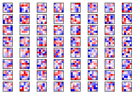
下面展示了一些第二个卷积层的权重(或滤波)。它们比第一个卷积层的权重更接近零,你可以看到比较低的标准差。
plot_conv_weights(weights=weights_conv2, input_channel=1)Min: -0.73326, Max: 0.25344
Mean: -0.00394, Stdev: 0.05466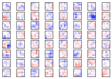
卷积层的输出
绘制图像的帮助函数。
def plot_image(image):
    # Create figure with sub-plots.
    fig, axes = plt.subplots(1, 2)

    # References to the sub-plots.
    ax0 = axes.flat[0]
    ax1 = axes.flat[1]

    # Show raw and smoothened images in sub-plots.
    ax0.imshow(image, interpolation='nearest')
    ax1.imshow(image, interpolation='spline16')

    # Set labels.
    ax0.set_xlabel('Raw')
    ax1.set_xlabel('Smooth')

    # Ensure the plot is shown correctly with multiple plots
    # in a single Notebook cell.
    plt.show()
绘制一张测试集中的图像。未处理的像素图像作为神经网络的输入。
img, cls = get_test_image(16)
plot_image(img)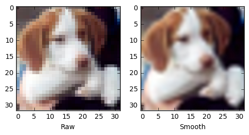
将原始图像作为神经网络的输入,然后画出第一个卷积层的输出。
plot_layer_output(output_conv1, image=img)
将同样的图像作为输入,画出第二个卷积层的输出。
plot_layer_output(output_conv2, image=img)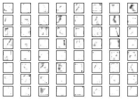
预测的类别标签
获取图像的预测类别标签和类别号。
label_pred, cls_pred = session.run([y_pred, y_pred_cls],
                                   feed_dict={x: [img]})
打印预测类别标签。
# Set the rounding options for numpy.
np.set_printoptions(precision=3, suppress=True)

# Print the predicted label.
print(label_pred[0])
[ 0. 0. 0. 0.493 0. 0.49 0.006 0.01 0. 0. ]
预测类别标签是长度为10的数组,每个元素代表着神经网络有多大信心认为图像是该类别。
在这个例子中,索引3的值是0.493,5的值为0.490。这表示神经网络相信图像要么是类别3,要么是类别5,即猫或狗。
class_names[3]'cat'
class_names[5]'dog'
关闭TensorFlow会话
现在我们已经用TensorFlow完成了任务,关闭session,释放资源。
# This has been commented out in case you want to modify and experiment
# with the Notebook without having to restart it.
# session.close()
结论
这篇教程介绍了如何创建一个在CIRAR-10数据集上进行图像分类的卷积神经网络。测试集上的分类准确率大概79-80%。
同时也画出了卷积层的输出,但很难看出神经网络如何分辨并分类图像。需要更好的可视化技巧。
练习
下面使一些可能会让你提升TensorFlow技能的一些建议练习。为了学习如何更合适地使用TensorFlow,实践经验是很重要的。
在你对这个Notebook进行改变之前,可能需要先备份一下。
- 执行10,000次迭代,看看分类准确率如何。将会保存一个checkpoint来储存TensorFlow图的所有变量。
- 再执行100,000次迭代,看看分类准确率有没有提升。然后再执行100,000次。准确率有提升吗,你认为值得这些增加的计算时间吗?
- 试着再预处理阶段改变图像的变体。
- 试着改变神经网络的结构。你可以让神经网络更大或更小。这对训练时间或分类准确率有什么影响?要注意的是,当你改变了神经网络结构时,就无法重新载入checkpoints了。
- 试着在第二个卷积层使用batch-normalization。也试试在俩个层中都删掉它。
- 研究一些CIFAR-10上的更好的神经网络 ,试着实现它们。
- 向朋友解释程序如何工作。
