关于pow的优化

球形高斯近似

之前提到，这篇文章介绍了通过 球形高斯近似 来优化 pow 的计算，代码如下：

优化前：

// Generalized Power Function
float pow(float x, float n)
{
    return exp(log(x) * n);
}

优化后：

// Spherical Gaussian Power Function 
float pow(float x, float n)
{
    n = n * 1.4427f + 1.4427f; // 1.4427f --> 1/ln(2)
    return exp2(x * n - n);
}

推导

关于上面代码的推导，可以参考这篇文章，这里再列一下主要推导过程：

pow 的 球形高斯近似:

pow(nh, K) = exp(-K*(1-nh))

其中 exp 可以用 exp2 这样表示：

exp(a) = exp2(a/ln(2))

带入后得到：

pow(nh, K) = exp2(-(K/ln(2))(1-nh))

这里的 1 / ln(2) 是一个常量，约等于 1.4427f，我们可以提前计算好，再带入上面的公式：

pow(nh, K) = exp2(-(K*1.4427f)(1-nh)) = exp2(nh*K*1.4427f-K*1.4427f)

把 K*1.4427 提出来后可以得到：

float A = K * 1.4427
pow(nh, K) = exp2(A * nh - A)

用代码表示如下：

// Spherical Gaussian Power Function 
float pow(float x, float n)
{
    n = n * 1.4427f;
    return exp2(x * n - n);
}

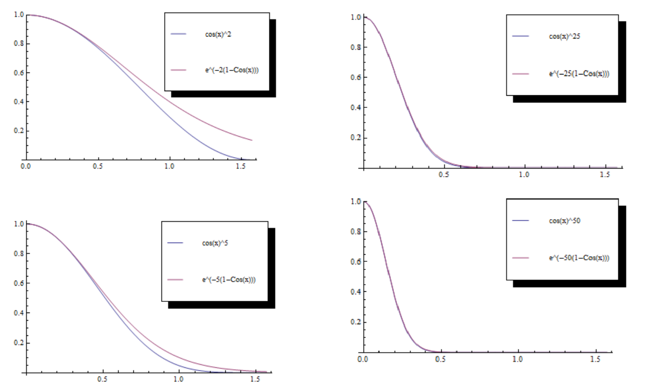
这个结果和文章最开头的优化代码还是有区别的，主要原因是 pow(nh, K) = exp(-K(1-nh))* 这个近似对于 比较小的K 来说近似结果相差较大，作者做了一些对比，如下图：

针对这个问题，作者也介绍了一个更好的近似方式，即给原先的公式添加一个常数，如下：

pow(nh, K) = exp((K+X)(nh-1))

可以看到，这里的 X 为 0 的时候就是之前的近似公式，作者建议 X 在 [0,1] 这个区间取值。

当 X 为 1 时，就是我们上面的优化代码：

// Spherical Gaussian Power Function 
float pow(float x, float n)
{
    n = n * 1.4427f + 1.4427f; // 1.4427f --> 1/ln(2)
    return exp2(x * n - n);
}

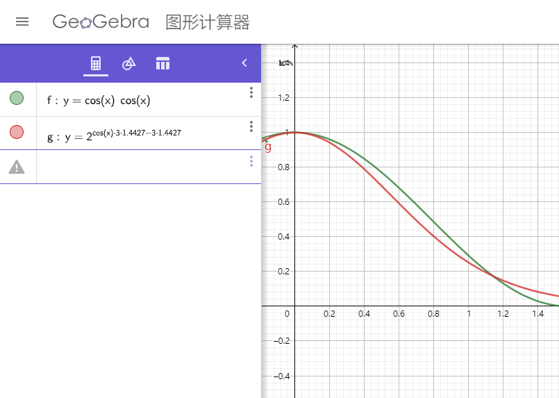
下图是添加常数后 pow(cos(x), 2) 的近似效果对比，红色曲线是近似曲线，可以看到，近似效果还不错：

游戏里的效果

优化前：

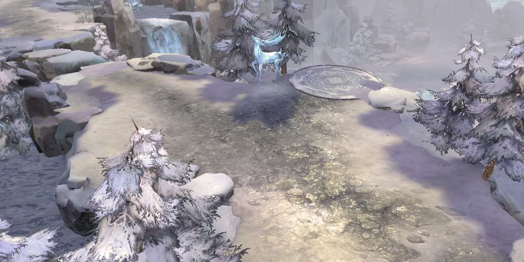
优化后：

地表的高光几乎看不出什么差别。

其他

作者的总结：

This post provided an application of a SG approximation, where the goal was to save a few ALU instructions. Again, for modern GPUs, this is not necessarily beneficial, but for older mainstream hardware, such as the PS3 and XBOX360 GPUs, it is a quite useful tool to have in your pocket.

意思是对于现代 GPU，这样做可能意义不大，不过对于老一点的硬件，这个优化值得拥有。

个人主页

本文的个人主页链接：baddogzz.github.io/2020/03/04/…。

好了，拜拜！